mlff_pattern_classification

Chapter 13: Data Mining > mlff_pattern_classification

mlff_pattern_classification

Calculates classifications for trained multilayered feedforward neural networks.

Synopsis

#include <imsls.h>

float *imsls_f_mlff_pattern_classification (
Imsls_f_NN_Network *network, int n_patterns,
int n_nominal, int n_continuous, int nominal[],
float continuous[], ..., 0)

The type double function is imsls_d_mlff_pattern_classification.

Required Arguments

Imsls_f_NN_Network *network (Input)
Pointer to a structure of type Imsls_f_NN_Network containing the trained feedforward network. See imsls_f_mlff_network.

int n_patterns (Input)
Number of patterns to classify.

int n_nominal (Input)
Number of nominal input attributes.

int n_continuous (Input)
Number of continuous attributes, including ordinal attributes encoded using cumulative percentage.

int nominal[] (Input)
Array of size n_patterns by n_nominal containing the nominal input variables.

float continuous[] (Input)
Array of size n_patterns by n_continuous containing the continuous and scaled ordinal input variables.

Return Value

Pointer to an array of size n_patterns by n_classes containing the predicted class probabilities associated with each input pattern, where n_classes is the number of possible target classifications. n_classes = network->n_outputs for non-binary classification categories. For binary classification, n_classes = 2. This space can be released by using the imsls_free function.

Synopsis with Optional Arguments

#include <imsls.h>

float *imsls_f_mlff_pattern_classification (Imsls_f_NN_Network *network, int n_patterns, int n_nominal, int n_continuous, int nominal[], float continuous[],
IMSLS_LOGISTIC_TABLE,
IMSLS_PREDICTED_CLASS, int **pred_class,
IMSLS_PREDICTED_CLASS_USER, int pred_class[],
IMSLS_RETURN_USER, float class_prob[],
0)

Optional Arguments

IMSLS_LOGISTIC_TABLE (Input)
This option specifies that all logistic activation functions are calculated using the table lookup approximation. This is only needed when a network is trained with this option and Stage II training is bypassed. If Stage II training was not bypassed during network training, weights were based upon the optimum network from Stage II which never uses a table lookup approximation to calculate logistic activations.

IMSLS_PREDICTED_CLASS int **pred_class (Output)
The address of a pointer to an array of size n_patterns containing the predicted classification for each pattern.

IMSLS_PREDICTED_CLASS_USER int pred_class[] (Output)
Storage for array pred_class provided by user. See IMSLS_PREDICTED_CLASS.

IMSLS_RETURN_USER, float class_prob[] (Output)
If specified, the classification probabilities for the input patterns are stored in the two-dimensional matrix class_prob of size n_patterns by n_classes, where n_classes is the number of target classes used to train the network. For binary classification problems, n_classes = 2. For all others,
n_classes = n_outputs = network->n_outputs.

Description

Function imsls_f_mlff_pattern_classification calculates classification probabilities from a previously trained multilayered feedforward neural network using the same network structure and scaling applied during the training. The structure Imsls_f_NN_Network describes the network structure used to originally train the network. The weights, which are the key output from training, are used as input to this function. The weights are stored in the Imsls_f_NN_Network structure.

In addition, two two-dimensional arrays are used to describe the values of the nominal and continuous attributes that are to be used as network inputs for calculating classification probabilities. Optionally, it can also return the predicted classifications in pred_class. The predicted classification is the target class with the highest probability, class_prob.

Function imsls_f_mlff_pattern_classification returns classification probabilities for the network input patterns.

Pattern Classification Attributes

Neural network classification inputs consist of the following types of attributes:

1. nominal attributes, and

2. continuous attributes, including ordinal attributes encoded to cumulative percentages.

The first data type contains the encoding of any nominal input attributes. If binary encoding is used, this encoding consists of creating columns of zeros and ones for each class value associated with every nominal attribute. The function imsls_f_unsupervised_nominal_filter can be used for this encoding.

When only one nominal attribute is used for input, then the number of binary encoded columns is equal to the number of classes for that attribute. If more nominal attributes appear in the data, then each nominal attribute is associated with several columns, one for each of its classes. Each column consists of zeros and ones. The column value is zero if that classification is not associated with this pattern; otherwise, it is equal to one if it is assigned to this pattern.

Consider an example with one nominal variable and two classes: male and female and the following five patterns: male, male, female, male, female. With binary encoding, the following 5 by 2 matrix is sent to the pattern classification to request classification probabilities for these patterns:

The second category of input attributes corresponds to continuous attributes. They are passed to this classification function via the floating point array continuous. The number of rows in this matrix is n_patterns, and the number of columns is n_continuous, corresponding to the number of continuous input attributes.

Ordinal input attributes, if used, are typically encoded to cumulative percentages. Since these are floating point values, they are placed into a column of the continuous array and n_continuous is set equal to the number of columns in this array.

In some cases, one of these types of input attributes may not exist. In that case, either
n_nominal = 0 or n_continuous = 0 and their corresponding input matrix is ignored.

Network Configuration

The configuration of the network consists of a description of the number of perceptrons for each layer, the number of hidden layers, the number of inputs and outputs, and a description of the linkages among the perceptrons. This description is passed into this training routine through the structure Imsls_f_NN_Network. See imsls_f_mlff_network. For binary problems there is only a single output since the probability P(class = 0) is equal to 1-P(class = 1). For other classification problems, however, n_outputs = n_classes and P(class = j) is equal to the classification probabilities in the j + 1 column of class_prob[].

Classification Probabilities

Classification probabilities are calculated from the input attributes, network structure and weights provided in network.

Classification probabilities are returned in a two-dimensional array, class_prob, with n_patterns rows and n_classes columns. The values in the i-th column are estimated probabilities for the class = (i-1).

Examples

Example 1

Fisher’s (1936) Iris data is often used for benchmarking discriminant analysis and classification solutions. It is part of the IMSL data sets and consists of the following continuous input attributes and classification target:

Continuous Attributes – X₁(sepal length), X₂(sepal width), X₃(petal length), and X₄(petal width)

Classification Target (Iris Type) – Setosa, Versicolour or Virginica.

The input attributes were scaled to z-scores using imsls_f_scale_filter. The hidden layer contained only 2 perceptrons and the output layer consisted of three perceptrons, one for each classification target.

Example 2 for imsls_f_mlff_classification_trainer used the following network structure for the 150 patterns in these data:

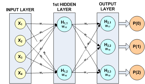
Figure 13- 16: A 2-layer, Classification Network with 4 Inputs 5 Perceptrons and a Target Classification with 3 Classes

imsls_f_mlff_classification_trainer found the following 19 weights for this network:

W₁ = -0.109866 W₂ = -0.0534655 W₃ = 4.92944 W₄ = -2.04734

W₅ = 10.2339 W₆ = -1495.09 W₇ = 3336.49 W₈ = 7372.98

W₉ = -9143.53 W₁₀ = 48.8937 W₁₁ = 240.958 W₁₂ = -3386.21

W₁₃ = 8904.6 W₁₄ = 3339.1 W₁₅ = 0.874638 W₁₆ = -7978.42

W₁₇ = 4586.22 W₁₈ = 1931.89 W₁₉ = -6518.14

The association of these weights with the calculation of the potentials for each perceptron is described in the following table:

PERCEPTRON	POTENTIAL	ACTIVATION
H_1,1	W15 + X1W1 + X2W2 + X3W3 + X4W4	LOGISTIC
H_1,2	W16 + X1W5 + X2W6 + X3W7 + X₄W8	LOGISTIC
H_2,1	W17 + H1,1W9 + H1,2W10	SOFTMAX
H_2,2	W18 + H_1,1W₁₁ + H1,2W12	SOFTMAX
H_2,3	W19 + H1,1W13 + H1,2W14	SOFTMAX

Table 13- 7 - Association of Network Weights with Perceptron Calculations

The potential calculations for each perceptron are activated using the assigned activation function. In this example, default activations were used, e.g. logistic for H1,1 and H1,2 and softmax for the output perceptrons H2,1, H2,2 and H2,3.

Note that in this case the network weights were retrieved from a file named iris_classfication.txt using imsls_f_mlff_network_read. This retrieves the trained network from mlff_classification_trainer described in Example 2. These were passed directly to imsls_f_mlff_pattern_classification in the Imsls_f_NN_Network structure.

#include <stdio.h>

#include <imsls.h>

/* ********************************************************************

* Three Layer Feed-Forward Network with 4 inputs, all

* continuous, and 3 classification categories.

* This is perhaps the best known database to be found in the pattern

* recognition literature. Fisher's paper is a classic in the

* field. The data set contains 3 classes of 50 instances each,

* where each class refers to a type of iris plant. One class is

* linearly separable from the other 2; the latter are NOT linearly

* separable from each other.

* Predicted attribute: class of iris plant.

* 1=Iris Setosa, 2=Iris Versicolour, and 3=Iris Virginica

* Input Attributes (4 Continuous Attributes)

* X1: Sepal length,

* X2: Sepal width,

* X3: Petal length,

* and X4: Petal width

**********************************************************************/

int main(){

float *classProb;

int i, j;

int n_patterns =150;

int n_inputs =4; /* four inputs, all continuous */

int n_nominal =0; /* no nominal input attributes */

int n_continuous =4; /* one continuous input attribute */

int n_outputs =3; /* total number of output perceptrons */

int *predicted_class;

int act_fcn[3] = {1, 1, 1};

int classification[150];

float unscaledX[150], scaledX[150];

float contAtt[4*150];

float *irisData;

float mean[4], s[4], center, spread;

char *colLabels[] = {"Pattern", "Class=0", "Class=1", "Class=2"};

char filename[] = "iris_classification.txt";

char prtLabel[] ="\nPredicted_Class | P(0) P(1) P(2)";

char dashes[] = "-----------------------------------------------";

/* Declare mlff network structure */

Imsls_f_NN_Network *network;

printf("******************************************************\n");

printf(" IRIS CLASSIFICATION EXAMPLE - PATTERN CLASSIFICATION \n");

printf("******************************************************\n");

irisData = imsls_f_data_sets(3,0);

* Setup the continuous attribute input array, contAtt[], and the

* network target classification array, classification[], using

* the above raw data matrix.

for(i=0; i < n_patterns; i++){

classification[i] = (int)irisData[i*5]-1;

for(j=1; j<5; j++){

contAtt[i*4+j-1] = irisData[i*5+j];

}

/* Scale continuous input attributes using z-score method */

for(j=0; j<n_continuous; j++){

for(i=0; i<n_patterns; i++)

unscaledX[i] = contAtt[i*n_continuous+j];

imsls_f_scale_filter(n_patterns, unscaledX, 2,

IMSLS_RETURN_USER, scaledX,

IMSLS_RETURN_CENTER_SPREAD, &center, &spread, 0);

for(i=0; i<n_patterns; i++)

contAtt[i*n_continuous+j] = scaledX[i];

mean[j] = center;

s[j] = spread;

}

printf("Scale Parameters: \n");

for(j=0; j<n_continuous; j++){

printf("Var %d Mean = %f S = %f \n",j+1, mean[j], s[j]);

}

network = imsls_f_mlff_network_read(filename, IMSLS_PRINT,0);

/* Use pattern classification routine to classify training

* patterns using trained network.

classProb = imsls_f_mlff_pattern_classification (network,

n_patterns, n_nominal, n_continuous, NULL, contAtt,

IMSLS_PREDICTED_CLASS, &predicted_class, 0);

/* Print class predictions */

printf("\n%s\n",prtLabel);

printf("%s\n",dashes);

for(i=0; i<n_patterns; i++){

printf(" %d ", predicted_class[i]);

printf(" | %f %f %f \n", classProb[i*3], classProb[i*3+1],

classProb[i*3+2]);

if(i==49 || i==99){

printf("\n%s\n",prtLabel);

printf("%s\n",dashes);

}

Output

The output for this example reproduces the 100% classification accuracy found during network training. For details, see Example 2 of imsls_f_mlff_classification_trainer.

******************************************************

IRIS CLASSIFICATION EXAMPLE - PATTERN CLASSIFICATION

******************************************************

Scale Parameters:

Var 1 Mean = 5.843334 S = 0.828065

Var 2 Mean = 3.057333 S = 0.435866

Var 3 Mean = 3.758000 S = 1.765298

Var 4 Mean = 1.199333 S = 0.762238

Attempting to open iris_classification.txt for

reading network data structure

File iris_classification.txt Successfully Opened

File iris_classification.txt closed

Predicted_Class | P(0) P(1) P(2)

-----------------------------------------------

0 | 1.000000 0.000000 0.000000

Predicted_Class | P(0) P(1) P(2)

-----------------------------------------------

1 | 0.000000 1.000000 0.000000

1 | 0.000000 0.999999 0.000001

1 | 0.000000 1.000000 0.000000

1 | 0.000000 0.999994 0.000006

1 | 0.000000 1.000000 0.000000

1 | 0.000000 0.999994 0.000006

1 | 0.000000 1.000000 0.000000

1 | 0.000002 0.999998 0.000000

1 | 0.000000 1.000000 0.000000

Predicted_Class | P(0) P(1) P(2)

-----------------------------------------------

2 | 0.000000 0.000000 1.000000

2 | 0.000000 0.000011 0.999989

2 | 0.000000 0.000000 1.000000

Example 2

Pattern classification is often used for pattern recognition, including playing simple games such as tic-tac-toe. The University of California at Irvine maintains a repository of data mining data, http://kdd.ics.uci.edu/. One consists of 958 patterns for board positions in tic-tac-toe donated by David Aha. See http://archive.ics.uci.edu/ml/datasets/Tic-Tac-Toe+Endgame for access to the actual data.

Each of the 958 patterns is described by nine nominal input attributes and one classification target. The nine nominal input attributes are the nine board positions in the game. Each has three classifications: X occupies the position, O occupies the position and vacant.

The target class is binary. A value of one indicates that the X player has one of eight possible wins in the next move. A value of zero indicates that this player does not have a winning position. 65.3% of the 958 patterns have a class = 1.

The nine nominal input attributes are mapped into 27 binary encoded columns, three for each of the nominal attributes. This makes a total of 27 input columns for the network. In this example, a neural network with one hidden layer containing ten perceptrons was found to provide 100% classification accuracy. This configuration is illustrated in the following figure.

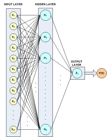
Figure 13- 17: A 2-layer, Binary Classification Network for Playing Tic-Tac-Toe

All hidden layer perceptrons used the default activation, logistic, and since the classification target is binary only one perceptron with logistic activation is used to calculate the probability of a loss for X, i.e. P(class = 0). All logistic activations are calculated using the IMSLS_LOGISTIC_TABLE option, which can reduce Stage I training time. Since Stage II training is bypassed, this option must also be used with the imsls_f_mlff_pattern_classification routine. This is the only time this option is used. If Stage II training was part of the network training, the final network weights would have been calculated without using the logistic table to approximate the calculations.

This structure results in a network with 27× 8 + 8 + 9 = 233 weights. It is surprising that with this small a number of weights relative to the number of training patterns, the trained network achieves 100% classification accuracy.

Unlike Example 1 in which the network was trained previously and retrieved using imsls_f_mlff_network_read, this example first trains the network and then passes the network structure network into imsls_f_mlff_pattern_classification.

#include <stdio.h>

#include <stdlib.h>

#include <imsls.h>

int main (){

int i, j, k, m, n_patterns, n_var;

int n_cat =9; /* 9 nominal input attributes */

int n_categorical =27; /* 9 Encoded = 27 categorical inputs */

int n_classes =2; /* positive or negative */

float *classProb;

float *trainStats;

int *predictedClass;

int classification[958];

float *inputData;

int *categoricalAtt, *nomTempIn, *nomTempOut, nClass;

Imsls_f_NN_Network *network;

/* get tic tac toe data */

inputData = imsls_f_data_sets (10,

IMSLS_N_OBSERVATIONS, &n_patterns,

IMSLS_N_VARIABLES, &n_var, 0);

printf("\n\n");

printf("*******************************************************\n");

printf("* TIC-TAC-TOE BINARY CLASSIFICATION EXAMPLE *\n");

printf("*******************************************************\n");

/* allocate memory for categoricalATT array */

categoricalAtt = (int*)malloc(958*n_categorical*sizeof(int));

/* populate categorical Att from catAtt using binary encoding */

nomTempIn = (int*) malloc(n_patterns*sizeof(int));

m=0;

for(i=0; i<n_cat; i++)

{

for(j=0; j<n_patterns; j++)

nomTempIn[j] = (int) inputData[j*n_var+i]+1;

nomTempOut =

imsls_unsupervised_nominal_filter(n_patterns, &nClass,

nomTempIn, 0);

for(k=0; k<nClass; k++)

{

for(j=0; j<n_patterns; j++)

categoricalAtt[j*n_categorical+m] = nomTempOut[j*nClass+k];

m++;

}

free(nomTempOut);

}

free(nomTempIn);

/* Setup the classification array, classification[] */

for(i=0; i < n_patterns; i++)

classification[i] = (int)inputData[(i*n_var)+n_var-1];

network = imsls_f_mlff_network_init(27, 1);

imsls_f_mlff_network(network, IMSLS_CREATE_HIDDEN_LAYER, 8,

IMSLS_LINK_ALL, 0);

imsls_random_seed_set(5555);

/* Train Classification Network */

trainStats = imsls_f_mlff_classification_trainer (network,

n_patterns, n_categorical, 0, classification, categoricalAtt,

NULL, IMSLS_STAGE_I, 30, n_patterns, IMSLS_NO_STAGE_II,

IMSLS_LOGISTIC_TABLE,

IMSLS_WEIGHT_INITIALIZATION_METHOD, IMSLS_EQUAL, 0);

* Use pattern classification routine to classify training patterns

* using trained network. This will reproduce the results returned

* in predicted_class[]

classProb = imsls_f_mlff_pattern_classification (network,

n_patterns, n_categorical, 0, categoricalAtt, NULL,

IMSLS_LOGISTIC_TABLE,

IMSLS_PREDICTED_CLASS, &predictedClass, 0);

/* Printing Classification Predictions */

printf("*******************************************************\n");

printf("Classification Minimum Cross-Entropy Error: %f\n",

trainStats[0]);

printf("Classification Error Rate: %f \n", trainStats[5]);

printf("*******************************************************\n");

printf("\nPRINTING FIRST TEN PREDICTIONS FOR EACH TARGET CLASS\n");

printf("*******************************************************\n");

printf(" |TARGET|PREDICTED| | *\n");

printf("PATTERN |CLASS | CLASS | P(class=0) | P(class=1) *\n");

printf("*******************************************************\n");

for(k=0; k<2; k++){

for(i=k*627; i<k*627+10; i++){

printf(" %d\t| %d | %d | ", i+1,

classification[i], predictedClass[i]);

printf("%f | %f \n",

classProb[i*n_classes], classProb[i*n_classes+1]);

}

printf("\n");

}

k=0;

for(i=0; i<n_patterns; i++)

if(classification[i] != predictedClass[i]) k++;

if(k==0) {

printf("All %d predicted classifications agree ", n_patterns);

printf("with target classifications\n");

}

Output

The output for this example demonstrates how imsls_f_mlff_pattern_classification reproduces the 100% classification accuracy found during network training.

*******************************************************

* TIC-TAC-TOE BINARY CLASSIFICATION EXAMPLE *

*******************************************************

Classification Minimum Cross-Entropy Error: 0.000022

Classification Error Rate: 0.000000

*******************************************************

PRINTING FIRST TEN PREDICTIONS FOR EACH TARGET CLASS

*******************************************************

|TARGET|PREDICTED| | *

PATTERN |CLASS | CLASS | P(class=0) | P(class=1) *

*******************************************************

1 | 1 | 1 | 0.000000 | 1.000000

2 | 1 | 1 | 0.000000 | 1.000000

3 | 1 | 1 | 0.000000 | 1.000000

4 | 1 | 1 | 0.000000 | 1.000000

5 | 1 | 1 | 0.000000 | 1.000000

6 | 1 | 1 | 0.000000 | 1.000000

7 | 1 | 1 | 0.000000 | 1.000000

8 | 1 | 1 | 0.000000 | 1.000000

9 | 1 | 1 | 0.000000 | 1.000000

10 | 1 | 1 | 0.000000 | 1.000000

628 | 0 | 0 | 1.000000 | 0.000000

629 | 0 | 0 | 1.000000 | 0.000000

630 | 0 | 0 | 1.000000 | 0.000000

631 | 0 | 0 | 1.000000 | 0.000000

632 | 0 | 0 | 1.000000 | 0.000000

633 | 0 | 0 | 1.000000 | 0.000000

634 | 0 | 0 | 1.000000 | 0.000000

635 | 0 | 0 | 1.000000 | 0.000000

636 | 0 | 0 | 1.000000 | 0.000000

637 | 0 | 0 | 1.000000 | 0.000000

All 958 predicted classifications agree with target classifications.

Contact Support