Usage Notes

This chapter includes routines for linear eigensystem analysis. Many of these are for matrices with special properties. Some routines compute just a portion of the eigensystem. Use of the appropriate routine can substantially reduce computing time and storage requirements compared to computing a full eigensystem for a general complex matrix.

An ordinary linear eigensystem problem is represented by the equation Ax = λx where A denotes an n × n matrix. The value λ is an eigenvalue and x ≠ 0 is the corresponding eigenvector. The eigenvector is determined up to a scalar factor. In all routines, we have chosen this factor so that x has Euclidean length with value one, and the component of x of smallest index and largest magnitude is positive. In case x is a complex vector, this largest component is real and positive.

Similar comments hold for the use of the remaining Level 1 routines in the following tables in those cases where the second character of the Level 2 routine name is no longer the character "2".

A generalized linear eigensystem problem is represented by Ax = λBx where A and B are n × n matrices. The value λ is an eigenvalue, and x is the corresponding eigenvector. The eigenvectors are normalized in the same manner as for the ordinary eigensystem problem. The linear eigensystem routines have names that begin with the letter “E”. The generalized linear eigensystem routines have names that begin with the letter “G”. This prefix is followed by a two-letter code for the type of analysis that is performed. That is followed by another two-letter suffix for the form of the coefficient matrix. The following tables summarize the names of the eigensystem routines.

 

Symmetric and Hermitian Eigensystems
	Symmetric Full	Symmetric Band	Hermitian Full
All eigenvalues	EVLSF	EVLSB	EVLHF
All eigenvalues and eigenvectors	EVCSF	EVCSB	EVCHF
Extreme eigenvalues	EVASF	EVASB	EVAHF
Extreme eigenvalues and eigenvectors	EVESF	EVESB	EVEHF
Eigenvalues in an interval	EVBSF	EVBSB	EVBHF
Eigenvalues and eigevectors in an interval	EVFSF	EVFSB	EVFHF
Performance index	EPISF	EPISB	EPIHF

 

General Eigensystems
	Real General	Complex General	Real Hessenberg	Complex Hessenberg
All eigenvalues	EVLRG	EVLCG	EVLRH	EVLCH
All eigenvalues and eigenvectors	EVCRG	EVCCG	EVCRH	EVCCH
Performance index	EPIRG	EPICG	EPIRG	EPICG

 

Generalized Eigensystems Ax = λBx
	Real General	Complex General	A Symmetric B Positive Definite
All eigenvalues	GVLRG	GVLCG	GVLSP
All eigenvalues and eigenvectors	GVCRG	GVCCG	GVCSP
Performance index	GPIRG	GPICG	GPISP

Error Analysis and Accuracy

The remarks in this section are for the ordinary eigenvalue problem. Except in special cases, routines will not return the exact eigenvalue-eigenvector pair for the ordinary eigenvalue problem Ax = λx. The computed pair

 

is an exact eigenvector-eigenvalue pair for a “nearby” matrix A + E. Information about E is known only in terms of bounds of the form ∥E∥2≤f(n)∥A∥2ɛ. The value of f(n) depends on the algorithm but is typically a small fractional power of n. The parameter ɛ is the machine precision. By a theorem due to Bauer and Fike (see Golub and Van Loan [1989, page 342]),

 

where σ(A) is the set of all eigenvalues of A (called the spectrum of A), X is the matrix of eigenvectors, ∥⋅∥2 is the 2-norm, and κ(X) is the condition number of X defined as κ(X) = ∥X∥2∥ X-1∥2. If A is a real symmetric or complex Hermitian matrix, then its eigenvector matrix X is respectively orthogonal or unitary. For these matrices, κ(X) = 1.

The eigenvalues

 

and eigenvectors

 

computed by EVC** can be checked by computing their performance index using EPI**. The performance index is defined by Smith et al. (1976, pages 124− 126) to be

 

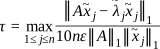
No significance should be attached to the factor of 10 used in the denominator. For a real vector x, the symbol ∥x∥1 represents the usual 1-norm of x. For a complex vector x, the symbol ∥x∥1 is defined by

 

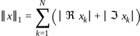
The performance index is related to the error analysis because

 

where E is the “nearby” matrix discussed above.

While the exact value of is machine and precision dependent, the performance of an eigensystem analysis routine is defined as excellent if  < 1, good if 1 ≤ ≤ 100, and poor if  > 100. This is an arbitrary definition, but large values of can serve as a warning that there is a blunder in the calculation. There are also similar routines GPI** to compute the performance index for generalized eigenvalue problems.

If the condition number κ(X) of the eigenvector matrix X is large, there can be large errors in the eigenvalues even if is small. In particular, it is often difficult to recognize near multiple eigenvalues or unstable mathematical problems from numerical results. This facet of the eigenvalue problem is difficult to understand: A user often asks for the accuracy of an individual eigenvalue. This can be answered approximately by computing the condition number of an individual eigenvalue. See Golub and Van Loan (1989, pages 344-345). For matrices A such that the computed array of normalized eigenvectors X is invertible, the condition number of λj is κj ≡ the Euclidean length of row j of the inverse matrix X-1. Users can choose to compute this matrix with routine LINCG, see Linear Systems. An approximate bound for the accuracy of a computed eigenvalue is then given by κjɛ∥A∥. To compute an approximate bound for the relative accuracy of an eigenvalue, divide this bound by ∣λj∣.