Bayesian seasonal adjustment modeling. The model allows for a decomposition of a time series into trend, seasonal, and an error component.
Required Arguments
W — Vector containing the stationary time series. (Input)
Optional Arguments
IORDER — Order of
trend differencing. (Input)
Default: IORDER = 2.
ISORDER — Order
of seasonal differencing. (Input)
Default: ISORDER =
1.
NFOCAST — Number
of forecasted values. (Input)
Default: NFOCAST = 0.
NPERIOD — Number
of seasonals within a period. (Input)
Default: NPERIOD = 12.
RIGID — Controls
rigidity of the seasonal pattern. (Input)
Default: RIGID = 1.0.
IPRINT — Printing option. (Input)
ABIC — The Akaike Bayesian Information Criterion for the estimated model. (Output)
TREND — Vector of length size(W)+ NFOCAST containing the estimated trend component for each data value followed by the trend estimates for the NFOCAST forecasted values. (Output)
SEASONAL — Vector of length size(W)+ NFOCAST containing the estimated seasonal components for each data value followed by the estimates for the NFOCAST forecasted seasonal values. (Output)
COMP — Vector of length size(W)containing the estimated irregular components. (Output)
SMOOTHED — Vector of length size(W)+ NFOCAST containing the estimated smoothed estimates for each of the time series values followed by the NFOCAST forecast values. (Output)
FORTRAN 90 Interface
Generic: CALL BAY_SEA (W [,…])
Specific: The specific interface names are S_BAY_SEA and D_BAY_SEA.
Description
Routine BAY_SEA is based upon the algorithm published by Akaike (1980). This algorithm uses a Bayesian approach to the problem of fitting the following autoregressive model for a time series Wt decomposed into a trend and a seasonal component.
Adopting the notation described earlier in the Usage Notes section of this chapter, if

then a seasonal autoregressive model can be represented by the following relationship:

where Wt
is the stationary time series with mean μ
, Tt denotes an
underlying trend, St
seasonal
component and At a noise or
irregular component.
A non-Bayesian approach to this problem would be to estimate the trend and seasonal components by minimizing

where p is the period of the seasonal component, and d, r , and z are properly chosen constants.
In BAY_SEA, the approach is to select the parameter d, which controls the smoothness of the trend and seasonality estimates, using Bayesian methods. The prior distribution controls the smoothness of the trend and seasonal components by assuming low order Gaussian autoregressive models for some differences of these components. The choice of the variance of the Gaussian distribution is realized by maximizing the log likelihood of the Bayesian model.
The other smoothing parameters, r and z, are determined by the value of RIGID. The default value for RIGID is 1. Larger values of RIGID produce a more rigid seasonal pattern. Normally, a series is first fit using the default value for RIGID. The smoothness of the trend and seasonality estimates are examined and then RIGID is either increased or decreased depending upon whether more or less seasonal smoothing is needed.
Additionally, BAY_SEA selects the optimum autoregressive model as the model that minimizes ABIC.
 ,
,where the likelihood in this case is the mixed
Bayesian maximum likelihood. Smaller values of represent a better fit.
Example
This example uses unadjusted unemployment for women over 20 years of age in the U.S. for 1991-2001, as reported by the U.S. Bureau of Labor Statistics (www.bls.gov). Figure 1 displays this data together with the smoothed preditions from BAY_SEA. Figure 2 displays the same data with trend predictions from BAY_SEA.
! SPECIFICATIONS FOR PARAMETERS
integer, parameter :: focast=12, nobs=132, nyears=11
data b/ 2968D0,3009D0,2962D0,2774D0,3040D0,3165D0,& !1991
3104D0,3313D0,3178D0,3142D0,3129D0,3107D0,&
3397D0,3447D0,3328D0,3229D0,3286D0,3577D0,& !1992
3799D0,3867D0,3655D0,3360D0,3310D0,3369D0,&
3643D0,3419D0,3108D0,3118D0,3146D0,3385D0,& !1993
3458D0,3468D0,3330D0,3244D0,3135D0,3005D0,&
3462D0,3272D0,3275D0,2938D0,2894D0,3106D0,& !1994
3150D0,3289D0,3136D0,2829D0,2776D0,2467D0,&
2944D0,2787D0,2749D0,2762D0,2578D0,2900D0,& !1995
3100D0,3102D0,2934D0,2864D0,2652D0,2456D0,&
3088D0,2774D0,2701D0,2555D0,2677D0,2741D0,& !1996
3052D0,2966D0,2772D0,2723D0,2705D0,2640D0,&
2898D0,2788D0,2718D0,2406D0,2520D0,2645D0,& !1997
2708D0,2811D0,2666D0,2380D0,2292D0,2187D0,&
2750D0,2595D0,2554D0,2213D0,2218D0,2449D0,& !1998
2532D0,2639D0,2449D0,2326D0,2302D0,2065D0,&
2447D0,2398D0,2381D0,2250D0,2086D0,2397D0,& !1999
2573D0,2475D0,2299D0,2054D0,2127D0,1935D0,&
2425D0,2245D0,2298D0,2005D0,2208D0,2379D0,& !2000
2459D0,2539D0,2182D0,1959D0,2012D0,1834D0,&
2404D0,2329D0,2285D0,2175D0,2245D0,2492D0,& !2001
2636D0,2892D0,2784D0,2771D0,2878D0,2856D0/
real(kind(1e0)) :: trend(nobs+focast), season(nobs+focast)
real(kind(1e0)) :: irreg(nobs), smooth(nobs+focast)
character :: months(focast)*3, years(nyears+2)*4
data months/'Jan', 'Feb', 'Mar', 'Apr', 'May', 'Jun', &
'Jul', 'Aug', 'Sep', 'Oct', 'Nov', 'Dec'/
data years/' ', '1991', '1992', '1993', '1994', '1995', &
'1996', '1997','1998','1999','2000','2001','2002'/
call bay_sea(b, trend=trend, seasonal=season, &
comp=irreg, abic=abicm, iorder=2, isorder=1,&
nfocast=focast, smoothed=smooth)
call wrrrl('TREND with last 12 values forecasted',trend,months, &
years, nra=12,nca=nyears+1,lda=12)
call wrrrl('SEASONAL with last 12 values forecasted',season,&
months,years, nra=12,nca=nyears+1, lda=12)
call wrrrl('IRREGULAR=Original data-TREND-SEASONAL',irreg, &
months,years, nra=12,nca=nyears,lda=12)
Output
TREND with last 12 values forecasted
1991 1992 1993 1994 1995 1996 1997 1998
Jan 2879.8 3318.9 3422.6 3228.7 2827.3 2795.7 2743.1 2481.3
Feb 2918.2 3359.9 3387.8 3206.0 2815.8 2785.6 2720.6 2469.7
Mar 2955.1 3399.1 3355.5 3177.0 2812.4 2777.9 2694.2 2455.4
Apr 2990.0 3436.1 3329.5 3142.1 2814.7 2773.2 2665.2 2439.0
May 3022.7 3469.0 3309.6 3103.9 2819.3 2771.3 2636.0 2422.8
Jun 3052.8 3496.1 3294.8 3064.8 2825.5 2771.0 2607.4 2408.5
Jul 3082.8 3514.5 3283.8 3025.7 2830.9 2772.4 2580.8 2396.8
Aug 3116.2 3521.9 3276.0 2987.3 2833.2 2773.6 2557.2 2387.7
Sep 3153.4 3517.8 3270.3 2949.0 2831.7 2774.7 2536.3 2380.3
Oct 3193.8 3503.7 3264.8 2911.3 2826.1 2774.5 2518.0 2373.6
Nov 3235.6 3482.4 3256.8 2876.6 2816.6 2770.4 2503.0 2366.6
Dec 3277.6 3455.2 3245.3 2847.6 2805.9 2760.2 2491.5 2359.1
Jan 2352.1 2235.9 2206.0 3166.1
Feb 2345.6 2237.6 2239.0 3275.1
Mar 2338.1 2239.3 2281.4 3384.1
Apr 2328.3 2238.9 2333.1 3493.0
May 2315.5 2235.2 2393.9 3602.0
Jun 2301.4 2226.3 2464.7 3710.9
Jul 2286.0 2212.8 2545.7 3819.9
Aug 2269.8 2196.6 2636.7 3928.9
Sep 2255.5 2181.3 2735.7 4037.8
Oct 2244.6 2171.9 2840.4 4146.8
Nov 2238.3 2172.1 2948.2 4255.8
Dec 2235.6 2183.3 3057.2 4364.7
SEASONAL with last 12 values forecasted
1991 1992 1993 1994 1995 1996 1997 1998 1999
Jan 162.9 165.6 169.3 172.0 173.8 176.3 176.4 177.3 176.4
Feb 51.4 51.5 50.5 49.5 48.6 48.8 50.0 51.1 51.0
Mar -24.0 -23.9 -23.4 -18.8 -16.3 -13.0 -8.7 -4.9 -3.0
Apr -191.0 -190.1 -189.1 -188.0 -186.6 -187.8 -188.5 -187.9 -186.6
May -140.6 -143.3 -145.4 -147.4 -148.1 -147.1 -147.1 -147.9 -147.7
Jun 67.2 66.6 65.8 64.4 63.3 62.2 62.7 63.6 64.9
Jul 176.9 180.1 181.6 183.0 185.5 186.6 185.8 186.1 187.2
Aug 251.9 253.0 252.6 253.3 253.1 252.8 253.7 254.4 255.2
Sep 76.4 77.2 77.1 77.3 75.5 73.3 72.6 70.7 68.9
Oct -79.5 -80.5 -80.1 -80.8 -81.5 -84.3 -87.6 -90.1 -93.4
Nov -119.8 -120.7 -120.5 -120.2 -120.4 -119.7 -119.7 -118.1 -117.6
Dec -235.7 -237.9 -243.0 -247.9 -250.5 -251.2 -254.2 -256.2 -257.5
IRREGULAR=Original data-TREND-SEASONAL
1991 1992 1993 1994 1995 1996 1997 1998 1999
Jan -74.7 -87.5 51.1 61.2 -57.1 116.0 -21.5 91.4 -81.5
Feb 39.4 35.6 -19.3 16.5 -77.4 -60.4 17.3 74.2 1.5
Mar 30.9 -47.2 -224.1 116.8 -47.1 -63.9 32.5 103.5 45.9
Apr -25.0 -17.0 -22.5 -16.1 133.9 -30.5 -70.6 -38.0 108.3
May 157.8 -39.7 -18.2 -62.6 -93.1 52.8 31.2 -56.9 -81.9
Jun 45.0 14.3 24.4 -23.1 11.2 -92.1 -25.1 -23.2 30.7
Jul -155.6 104.4 -7.4 -58.6 83.6 93.0 -58.6 -50.9 99.9
Aug -55.0 92.1 -60.6 48.4 15.7 -60.4 0.1 -3.1 -49.9
Sep -51.8 60.0 -17.4 109.6 26.8 -76.0 57.1 -2.1 -25.3
Oct 27.7 -63.3 59.3 -1.5 119.4 32.8 -50.3 42.5 -97.1
Nov 13.2 -51.7 -1.3 19.5 -44.3 54.3 -91.3 53.5 6.3
Dec 65.1 151.7 2.7 -132.8 -99.4 131.0 -50.3 -37.9 -43.1
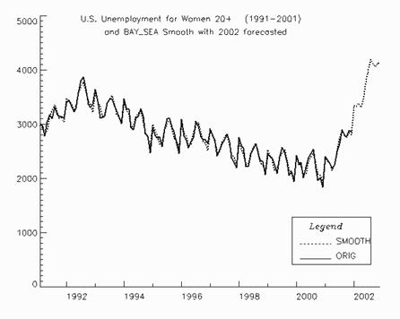
Figure 8-4 Sample Smoothed Predictions from BAY_SEA
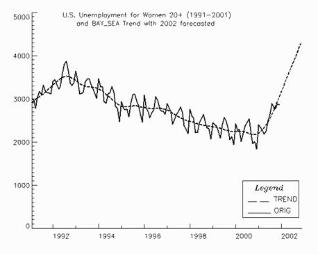
Figure 8- 5 Sample Trend Predictions from BAY_SEA
|
Visual Numerics, Inc. PHONE: 713.784.3131 FAX:713.781.9260 |