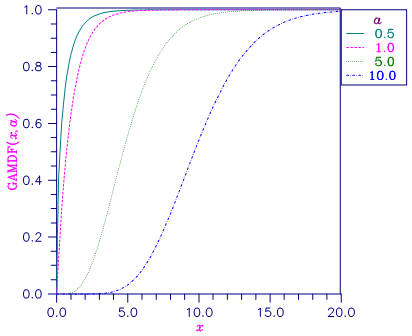
This function evaluates the gamma cumulative distribution function.

Function Return Value

GAMDF — Function value, the probability that a gamma random variable takes a value less than or equal to X.   (Output)

Required Arguments

X — Argument for which the gamma distribution function is to be evaluated.   (Input)

A — The shape parameter of the gamma distribution.   (Input)
This parameter must be positive.

FORTRAN 90 Interface

Generic:                              GAMDF (X, A)

Specific:                             The specific interface names are S_GAMDF and D_GAMDF.

FORTRAN 77 Interface

Single:                                GAMDF (X, A)

Double:                              The double precision name is DGAMDF.

Description

Function GAMDF evaluates the distribution function, F, of a gamma random variable with shape parameter a; that is,

 

 

where Γ(⋅) is the gamma function. (The gamma function is the integral from 0 to ∞ of the same integrand as above). The value of the distribution function at the point x is the probability that the random variable takes a value less than or equal to x.

The gamma distribution is often defined as a two-parameter distribution with a scale parameter b (which must be positive), or even as a three-parameter distribution in which the third parameter c is a location parameter. In the most general case, the probability density function over (c, ∞) is

 

If T is such a random variable with parameters a, b, and c, the probability that T ≤ t0 can be obtained from GAMDF by setting X = (t0 − c)/b.

If X is less than a or if X is less than or equal to 1.0, GAMDF uses a series expansion. Otherwise, a continued fraction expansion is used. (See Abramowitz and Stegun, 1964.)

Figure 11- 11   Gamma Distribution Function

Comments

Informational error

Type Code

1         2                  Since the input argument X is less than zero, the distribution function is set to zero.

Example

Suppose X is a gamma random variable with a shape parameter of 4. (In this case, it has an Erlang distribution since the shape parameter is an integer.) In this example, we find the probability that X is less than 0.5 and the probability that X is between 0.5 and 1.0.

 

      USE UMACH_INT

      USE GAMDF_INT

      IMPLICIT   NONE

      INTEGER    NOUT

      REAL       A, P, X

!

      CALL UMACH (2, NOUT)

      A = 4.0

      X = 0.5

      P = GAMDF(X,A)

      WRITE (NOUT,99998) P

99998 FORMAT (' The probability that X is less than 0.5 is ', F6.4)

      X = 1.0

      P = GAMDF(X,A) - P

      WRITE (NOUT,99999) P

99999 FORMAT (' The probability that X is between 0.5 and 1.0 is ', &

            F6.4)

      END

Output

 

The probability that X is less than 0.5 is 0.0018
The probability that X is between 0.5 and 1.0 is 0.0172

http://www.vni.com/ PHONE: 713.784.3131 FAX:713.781.9260