Package com.imsl.stat

Class Pdf

java.lang.Object

com.imsl.stat.Pdf

public final class Pdf
extends Object

Probability density functions.

See Also:

• Example
• Cumulative distribution function
• Inverse Cumulative Distribution Function

Nested Class Summary

Nested Classes

Modifier and Type	Class	Description
static class	Pdf.AltSeriesAccuracyLossException	The magnitude of alternating series sum is too small relative to the sum of positive terms to permit a reliable accuracy.

Method Summary

Modifier and Type	Method	Description
static double	beta(double x, double pin, double qin)	Evaluates the beta probability density function.
static double	binomial(int k, int n, double p)	Evaluates the binomial probability density function.
static double	chi(double chsq, double df)	Evaluates the chi-squared probability density function
static double	continuousUniform(double x, double a, double b)	Evaluates the continuous uniform probability density function.
static double	discreteUniform(int x, int n)	Evaluates the discrete uniform probability density function.
static double	exponential(double x, double scale)	Evaluates the exponential probability density function
static double	extremeValue(double x, double mu, double beta)	Evaluates the extreme value probability density function.
static double	F(double x, double dfn, double dfd)	Evaluates the F probability density function.
static double	gamma(double x, double a, double b)	Evaluates the gamma probability density function.
static double	generalizedExtremeValue(double x, double mu, double sigma, double xi)	Evaluates the generalized extreme value probability density function.
static double	generalizedGaussian(double x, double mu, double alpha, double beta)	Evaluates the generalized Gaussian (normal) probability density function.
static double	generalizedPareto(double x, double mu, double sigma, double alpha)	Evaluates the generalized Pareto probability density function.
static double	geometric(int x, double p)	Evaluates the geometric probability density (or mass) function.
static double	hypergeometric(int k, int sampleSize, int defectivesInLot, int lotSize)	Evaluates the hypergeometric probability density function.
static double	inverseGaussian(double x, double mean, double lambda)	Evaluates the inverse Gaussian probability density function.
static double	logistic(double x, double mu, double sigma)	Evaluates the logistic probability density function.
static double	logLogistic(double x, double alpha, double beta)	Evaluates the Log-logistic probability density function.
static double	logNormal(double x, double mu, double sigma)	Evaluates the standard lognormal probability density function.
static double	negativeBinomial(int k, double r, double p)	Evaluates the negative binomial probability density function.
static double	noncentralBeta(double x, double shape1, double shape2, double lambda)	Evaluates the noncentral beta probability density function (PDF).
static double	noncentralChi(double chsq, double df, double alam)	Evaluates the noncentral chi-squared probability density function (PDF).
static double	noncentralF(double f, double df1, double df2, double lambda)	Evaluates the noncentral F probability density function (PDF).
static double	noncentralStudentsT(double t, double df, double delta)	Evaluates the noncentral Student's t probability density function.
static double	normal(double x, double mean, double stdev)	Evaluates the normal (Gaussian) probability density function.
static double	Pareto(double x, double xm, double k)	Evaluates the Pareto probability density function.
static double	poisson(int k, double theta)	Evaluates the Poisson probability density function.
static double	Rayleigh(double x, double sigma)	Evaluates the Rayleigh probability density function.
static double	Weibull(double x, double k, double lambda)	Evaluates the Weibull probability density function.

Methods inherited from class java.lang.Object

clone, equals, finalize, getClass, hashCode, notify, notifyAll, toString, wait, wait, wait

Method Details

noncentralBeta

public static double noncentralBeta(double x,
 double shape1,
 double shape2,
 double lambda)

Evaluates the noncentral beta probability density function (PDF).

The noncentral beta distribution is a generalization of the beta distribution. If \(Z\) is a noncentral chi-square random variable with noncentrality parameter \(\lambda\) and \(2 \alpha_1\) degrees of freedom, and \(Y\) is a chi-square random variable with \(2 \alpha_2\) degrees of freedom which is statistically independent of \(Z\), then

$$X \;\; = \;\; \frac{Z}{Z \; + \; Y} \;\; = \;\; \frac{\alpha_1 F}{\alpha_1 F \; + \; \alpha_2}$$

is a noncentral beta-distributed random variable and

$$F \;\; = \;\; \frac{\alpha_2 Z}{\alpha_1 Y} \;\; = \;\; \frac{\alpha_2 X}{\alpha_1 (1 \; - \; X)}$$

is a noncentral F-distributed random variable. The PDF for noncentral beta variable X can thus be simply defined in terms of the noncentral F PDF:

$$PDF_{nc\beta}(x, \; \alpha_1, \; \alpha_2, \; \lambda) \;\; = \;\; PDF_{ncF}(f, \; 2 \alpha_1, \; 2 \alpha_2, \; \lambda) \; \frac{df}{dx}$$

where \(PDF_{nc\beta}(x, \; \alpha_1, \; \alpha_2, \; \lambda)\) is the noncentral beta PDF with \(x\) = x, \(\alpha_1\) = shape1, \(\alpha_2\) = shape2, and noncentrality parameter \(\lambda\) = lambda; \(PDF_{ncF}(f, \; 2 \alpha_1, \; 2 \alpha_2, \; \lambda)\) is the noncentral F PDF with argument f, numerator and denominator degrees of freedom \(2 \alpha_1\) and \(2 \alpha_2\) respectively, and noncentrality parameter \(\lambda\); and $$\frac{df}{dx} \;\; = \;\; \frac{(\alpha_1 f \; + \; \alpha_2)^2}{\alpha_1 \alpha_2} \;\; = \;\; \frac{ \alpha_2}{\alpha_1 (1 \; - \; x)^2} $$ where $$f \;\; = \;\; \frac{\alpha_2 x}{\alpha_1 (1 \; - \; x)}$$ and $$x \;\; = \;\; \frac{\alpha_1 f}{\alpha_1 f \; + \; \alpha_2}$$

(See documentation for class Cdf method noncentralF for a discussion of how the noncentral F PDF is defined and calculated.)

With a noncentrality parameter of zero, the noncentral beta distribution is the same as the beta distribution.

Parameters:

x - a double scalar value representing the argument at which the function is to be evaluated. x must be nonnegative and less than or equal to 1.

shape1 - a double scalar value representing the first shape parameter. shape1 must be positive.

shape2 - a double scalar value representing the second shape parameter. shape2 must be positive.

lambda - a double scalar value representing the noncentrality parameter. lambda must nonnegative.

Returns:

a double scalar value representing the probability density associated with a noncentral beta random variable with value x.

binomial

public static double binomial(int k,
 int n,
 double p)

Evaluates the binomial probability density function.

Method binomial evaluates the probability that a binomial random variable with parameters n and p takes on the value k. It does this by computing probabilities of the random variable taking on the values in its range less than (or the values greater than) k. These probabilities are computed by the recursive relationship

$$\Pr \left( {X = j} \right) = \frac{{\left( {n + 1 - j} \right)p}}{{j\left( {1 - p} \right)}}\Pr \left( {X = j - 1} \right)$$

To avoid the possibility of underflow, the probabilities are computed forward from 0, if k is not greater than \(n \times p\), and are computed backward from n, otherwise. The smallest positive machine number, \(\varepsilon\), is used as the starting value for computing the probabilities, which are rescaled by \((1 - p)^n \varepsilon\) if forward computation is performed and by \(p^n\varepsilon\) if backward computation is done.

For the special case of p = 0, binomial is set to 0 if k is greater than 0 and to 1 otherwise; and for the case p = 1, binomial is set to 0 if k is less than n and to 1 otherwise.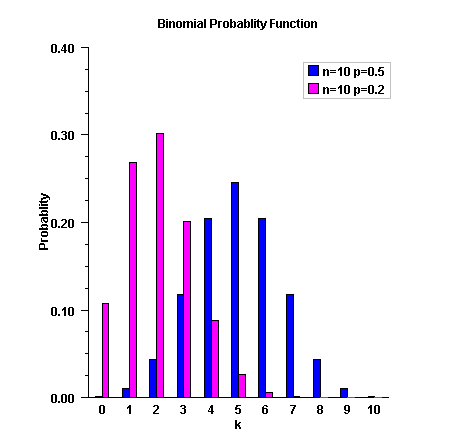

Parameters:

k - the int argument for which the binomial distribution function is to be evaluated.

n - the int number of Bernoulli trials.

p - a double scalar value representing the probability of success on each independent trial.

Returns:

a double scalar value representing the probability that a binomial random variable takes a value equal to k.

See Also:

• Example

poisson

public static double poisson(int k,
 double theta)

Evaluates the Poisson probability density function.

Method poisson evaluates the probability density function of a Poisson random variable with parameter theta. theta, which is the mean of the Poisson random variable, must be positive. The probability function (with \(\theta = theta\)) is

$$f(x) = e^{- \theta} \,\,\theta ^k /k!,\,\,\,\,\, for\,k = 0,\,\,1,\,\,2,\, \ldots$$

poisson evaluates this function directly, taking logarithms and using the log gamma function.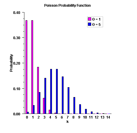

Parameters:

k - the int argument for which the Poisson probability function is to be evaluated.

theta - a double scalar value representing the mean of the Poisson distribution.

Returns:

a double scalar value representing the probability that a Poisson random variable takes a value equal to k.

See Also:

• Example

beta

public static double beta(double x,
 double pin,
 double qin)

Evaluates the beta probability density function.

Parameters:

x - a double, the argument at which the function is to be evaluated.

pin - a double, the first beta distribution parameter.

qin - a double, the second beta distribution parameter.

Returns:

a double, the value of the probability density function at x.

F

public static double F(double x,
 double dfn,
 double dfd)

Evaluates the F probability density function.

The probability density function of the F distribution is $${\it f}(x, {\it dfn}, {\it dfd})= {\frac { {\Gamma}(\frac {v_1 + v_2}{2})({\frac {v_1}{v_2})}^{\frac{v_1}{2}} x^{\frac {v_1}{2}} } {{{\Gamma}(\frac {v_1}{2}) }{{\Gamma}(\frac {v_2}{2}) } {(1+\frac{v_1x}{v_2})}^{\frac{v_1+v_2}{2} } }}$$ where \(v_1\) and \(v_2\) are the shape parameters dfn and dfd and \(\Gamma\) is the gamma function, $${\Gamma (a)} = {\int}_{0}^{\infty}{t^{a-1} e^{-t } \it dt}$$.

Parameters:

x - a double, the argument at which the function is to be evaluated.

dfn - a double, the numerator degrees of freedom. It must be positive.

dfd - a double, the denominator degrees of freedom. It must be positive.

Returns:

a double, the value of the probability density function at x.

hypergeometric

public static double hypergeometric(int k,
 int sampleSize,
 int defectivesInLot,
 int lotSize)

Evaluates the hypergeometric probability density function.

Method hypergeometric evaluates the probability density function of a hypergeometric random variable with parameters n, l, and m. The hypergeometric random variable X can be thought of as the number of items of a given type in a random sample of size n that is drawn without replacement from a population of size l containing m items of this type. The probability density function is:

$${\rm{Pr}}\left( {X = k} \right) = \frac{{\left( {_k^m } \right)\left( {_{n - k}^{l - m} } \right)}}{{\left( {_n^l } \right)}}{\rm{for}} \,\,\, k = i,\;i + 1,\,i + 2\; \ldots ,\;\min \left( {n,m} \right)$$

where i = max(0, n - l + m). hypergeometric evaluates the expression using log gamma functions.

Parameters:

k - an int, the argument at which the function is to be evaluated.

sampleSize - an int, the sample size, n.

defectivesInLot - an int, the number of defectives in the lot, m.

lotSize - an int, the lot size, l.

Returns:

a double, the probability that a hypergeometric random variable takes on a value equal to k.

See Also:

• Example

gamma

public static double gamma(double x,
 double a,
 double b)

Evaluates the gamma probability density function. The probability density function of the gamma distribution is

$$ f(x; a, b) = x^{a - 1} \frac{1}{{b^{a} \Gamma (a)}} e^{ - {x}/{b}} $$

where a is the shape parameter and b is the scale parameter.

Parameters:

x - a double scalar value representing the argument at which the function is to be evaluated.

a - a double scalar value representing the shape parameter. This must be positive.

b - a double scalar value representing the scale parameter. This must be positive.

Returns:

a double scalar value, the probability density function at x.

generalizedExtremeValue

public static double generalizedExtremeValue(double x,
 double mu,
 double sigma,
 double xi)

Evaluates the generalized extreme value probability density function.

The probability density function of the generalized extreme value distribution is $$f(x|\mu,\sigma,\xi)=\frac{1}{\sigma}t(x)^{\xi+1}e^{-t(x)}$$ where $$t(x)=\left\{\begin{array}{lll} (1+\xi(\frac{x-\mu}{\sigma}))^{-\frac{1}{\xi}}& \mbox{for} & \xi \ne 0 \\ e^{-\frac{x-\mu}{\sigma}} & \mbox{for} & \xi = 0 \end{array}\right. $$ \( \mu\in \mathbb{R} \) is the location parameter, \(\sigma > 0 \) is the scale parameter, and \(\xi \in \mathbb{R} \) is the shape parameter. Furthermore, the support for the distribution is $$\left\{\begin{array}{lll} x \in \mathbb{R} & \mbox{for} & \xi = 0 \\ x \ge \mu - \frac{\sigma}{\xi} & \mbox{for} & \xi > 0 \\ x \le \mu - \frac{\sigma}{\xi} & \mbox{for} & \xi \lt 0 \end{array}\right. $$

References
1. Wikipedia contributors. "Generalized extreme value distribution." Wikipedia, The Free Encyclopedia.

Parameters:

x - a double, the value (quantile) at which to evaluate the pdf

mu - a double, the value of the location parameter

sigma - a double, the value of the scale parameter

xi - a double, the value of the shape parameter

Returns:

a double, the value of the pdf evaluated at x given the parameter values

generalizedGaussian

public static double generalizedGaussian(double x,
 double mu,
 double alpha,
 double beta)

Evaluates the generalized Gaussian (normal) probability density function.

The generalized Gaussian probability density function is given by

$$ f(x; \mu,\alpha, \beta) = \frac{\beta}{2\alpha\Gamma(\frac{1}{\beta})} e^{-(\frac{|x-\mu|}{\alpha})^\beta} $$

where \(\mu\) is the location parameter, \(\alpha >0 \) is the scale parameter, and \(\beta >0 \) is the shape parameter. Note that this follows the parameterization given in Wikipedia. There are alternative parameterizations, as in Roenko, et. al. 2014.

References
1. Roenko, Alexey, Lukin, Vladimir, Djurovic, Igor, Simeunović, Marko. (2014). Estimation of parameters for generalized Gaussian distribution. ISCCSP 2014 - 2014 6th International Symposium on Communications, Control and Signal Processing, Proceedings. 376-379.
2. Wikipedia contributors. "Generalized normal distribution." Wikipedia, The Free Encyclopedia.

Parameters:

x - a double, the point at which the function is to be evaluated

mu - a double, the location parameter

alpha - a double, the scale parameter

beta - a double, the shape parameter

Returns:

a double, the probability density at x given the parameter values

generalizedPareto

public static double generalizedPareto(double x,
 double mu,
 double sigma,
 double alpha)

Evaluates the generalized Pareto probability density function. The generalized Pareto probability density function is given by $$ f(x; \mu,\sigma, \alpha) = \frac{1}{\sigma}\left( 1 + \frac{\alpha (x-\mu)}{\sigma}\right)^{(-\frac{1}{\alpha} - 1)} $$

where \(\mu \in \mathbb{R} \) is the location parameter, \(\sigma \gt 0 \) is the scale parameter, and \(\alpha \in \mathbb{R} \) is the shape parameter. Note that for \(\alpha=0\), the pdf is the limiting form of the above. The support for \(\alpha \ge 0\) is \( x \ge \mu \), while for \( \alpha \lt 0 \), \(\mu \le x \le \mu - \frac{\sigma}{\alpha}\). Note that this follows the parameterization given in Wikipedia.

References
1. Wikipedia contributors. "Generalized Pareto distribution." Wikipedia, The Free Encyclopedia.

Parameters:

x - a double, the point at which the function is to be evaluated

mu - a double, the location parameter

sigma - a double, the scale parameter. It must be positive.

alpha - a double, the shape parameter

Returns:

a double, the probability density at x given the parameter values

exponential

public static double exponential(double x,
 double scale)

Evaluates the exponential probability density function

Parameters:

x - a double scalar value representing the argument at which the function is to be evaluated.

scale - a double scalar value representing the scale parameter.

Returns:

a double scalar value, the value of the probability density function at x.

normal

public static double normal(double x,
 double mean,
 double stdev)

Evaluates the normal (Gaussian) probability density function.

The probability density function for a normal distribution is given by $$\frac{1}{\sigma \sqrt{2\pi}} {e}^{ \frac{{-(x - \mu)}^2}{{2 {\sigma}^2}} } $$ where \(\mu\) and \(\sigma\) are the mean and standard deviation.

Parameters:

x - a double scalar value representing the argument at which the function is to be evaluated.

mean - a double scalar value containing the mean.

stdev - a double scalar value containing the standard deviation.

Returns:

a double containing the value of the probability density function at x

chi

public static double chi(double chsq,
 double df)

Evaluates the chi-squared probability density function

Parameters:

chsq - a double scalar value representing the argument at which the function is to be evaluated.

df - a double scalar value representing the number of degrees of freedom. df must be positive.

Returns:

a double scalar value, the value of the probability density function at chsq.

noncentralChi

public static double noncentralChi(double chsq,
 double df,
 double alam)

Evaluates the noncentral chi-squared probability density function (PDF).

The noncentral chi-squared distribution is a generalization of the chi-squared distribution. If \(\{X_i\}\) are \(k\) independent, normally distributed random variables with means \(\mu_i\) and variances \(\sigma^2_i\), then the random variable

$$X \;\; = \;\; \sum_{i = 1}^k \left(\frac{X_i}{\sigma_i}\right)^2$$

is distributed according to the noncentral chi-squared distribution. The noncentral chi-squared distribution has two parameters, \(k\) which specifies the number of degrees of freedom (i.e. the number of \(X_i\)), and \(\lambda\) which is related to the mean of the random variables \(X_i\) by

$$\lambda \;\; = \;\; \sum_{i = 1}^k \left(\frac{\mu_i}{\sigma_i}\right)^2$$

The noncentral chi-squared distribution is equivalent to a (central) chi-squared distribution with \(k + 2i\) degrees of freedom, where \(i\) is the value of a Poisson distributed random variable with parameter \(\lambda/2\). Thus, the probability density function is given by:

$$F(x,k,\lambda) \;\; = \;\; \sum_{i = 0}^\infty {\frac{e^{-\lambda/2} (\lambda/2)^i}{i!}} f(x,k+2i)$$

where the (central) chi-squared PDF \(f(x, k)\) is given by:

$$f(x, k) \;\; = \;\; \frac{(x/2)^{k/2} \; e^{-x/2}}{x \; \Gamma(k/2)} \quad for \;\; x \; > \; 0, \;\; else \;\; 0$$

where \(\Gamma (\cdot)\) is the gamma function. The above representation of \(F(x,k,\lambda)\) can be shown to be equivalent to the representation:

$$F(x,k,\lambda) \;\; = \;\; \frac{e^{-(\lambda+x)/2} \; (x/2)^{k/2}}{x} \; \sum_{i = 0}^\infty {\phi_i}$$

$$\phi_i \;\; = \;\; \frac{(\lambda x / 4)^i}{i! \; \Gamma(k/2 \;\; + \;\; i)}$$

Method noncentralChi evaluates the probability density function, \(F(x,k,\lambda)\), of a noncentral chi-squared random variable with df degrees of freedom and noncentrality parameter alam, corresponding to k = df, \(\lambda\) = alam, and x = chsq.

Method noncentralChi evaluates the cumulative distribution function incorporating the above probability density function.

With a noncentrality parameter of zero, the noncentral chi-squared distribution is the same as the central chi-squared distribution.

Parameters:

chsq - a double scalar value at which the function is to be evaluated. chsq must be nonnegative.

df - a double scalar value representing the number of degrees of freedom. df must be positive.

alam - a double scalar value representing the noncentrality parameter. alam must be nonnegative.

Returns:

a double scalar value representing the probability density associated with a noncentral chi-squared random variable with value chsq.

noncentralStudentsT

public static double noncentralStudentsT(double t,
 double df,
 double delta)
                                  throws Pdf.AltSeriesAccuracyLossException

Evaluates the noncentral Student's t probability density function.

The noncentral Student's t-distribution is a generalization of the Student's t-distribution. If \(w\) is a normally distributed random variable with unit variance and mean \(\delta\) and \(u\) is a chi-square random variable with \(\nu\) degrees of freedom that is statistically independent of \(w\), then $$T \;\; = \;\; w/\sqrt{u/\nu}$$ is a noncentral t-distributed random variable with \(\nu\) degrees of freedom and noncentrality parameter \(\delta\), that is, with \(\nu\) = df, and \(\delta\) = delta. The probability density function for the noncentral t-distribution is: $$f(t,\nu,\delta) \;\; = \;\; \frac{\nu^{\nu/2} \; e^{-\delta^2/2}}{\sqrt{\pi} \; \Gamma(\nu/2) \; ( \nu + t^2 ) ^ {(\nu + 1)/2}} \; \sum_{i = 0}^\infty {\Phi_i}$$ where $$\Phi_i \;\; = \;\; \frac{\Gamma((\nu + i + 1)/2)}{i!} \; [\delta t]^i \; \left(\frac{2}{\nu + t^2}\right)^{i/2}$$ and t = t.

For noncentrality parameter \(\delta\) = 0, the PDF reduces to the (central) Student's t PDF: $$f(t,\nu,0) \;\; = \;\; \frac{\Gamma((\nu+1)/2) \; \left( 1 \; + \; (t^2/\nu) \right)^{-(\nu+1)/2}}{\sqrt{\nu \pi} \; \Gamma(\nu/2)}$$ and, for t = 0, the PDF becomes: $$f(0,\nu,\delta) \;\; = \;\; \frac{\Gamma((\nu+1)/2) \; e^{-\delta^2/2}}{\sqrt{\nu \pi} \; \Gamma(\nu/2)}$$ Method noncentralStudentsT evaluates the cumulative distribution function incorporating the above probability density function.

Parameters:

t - a double value representing the argument at which the function is to be evaluated.

df - a double value representing the number of degrees of freedom. df must be positive.

delta - a double value representing the noncentrality parameter.

Returns:

a double value representing the probability density associated with a noncentral Student's t random variable with value t.

Throws:

Pdf.AltSeriesAccuracyLossException - is thrown when the magnitude of alternating series sum is too small relative to the sum of positive terms to permit a reliable accuracy.

noncentralF

public static double noncentralF(double f,
 double df1,
 double df2,
 double lambda)

Evaluates the noncentral F probability density function (PDF).

The noncentral F distribution is a generalization of the F distribution. If \(x\) is a noncentral chi-square random variable with noncentrality parameter \(\lambda\) and \(\nu_1\) degrees of freedom, and \(y\) is a chi-square random variable with \(\nu_2\) degrees of freedom which is statistically independent of \(X\), then $$F \;\; = \;\; (x/\nu_1)/(y/\nu_2)$$ is a noncentral F-distributed random variable whose PDF is given by: $$PDF(f, \nu_1, \nu_2, \lambda) \;\; = \;\; \Psi \; \sum_{k = 0}^\infty {\Phi_k} $$ where $$\Psi \;\; = \;\; \frac{ e^{-\lambda/2}(\nu_1 f)^{\nu_1/2}(\nu_2)^{\nu_2/2} } { f \; (\nu_1 f \; + \; \nu_2)^{(\nu_1 + \nu_2)/2} \; \Gamma(\nu_2/2) }$$ $$\Phi_k \;\; = \;\; \frac{ R^k \; \Gamma(\frac{\nu_1 + \nu_2}{2} \; + \; k) } { k! \; \Gamma(\frac{\nu_1}{2} \; + \; k) } $$ $$R \;\; = \;\; \frac{ \lambda \nu_1 f }{ 2 (\nu_1 f \; + \; \nu_2)} $$ where \(\Gamma (\cdot)\) is the gamma function, \(\nu_1\) = df1, \(\nu_2\) = df2, \(\lambda\) = lambda, and f = f.

With a noncentrality parameter of zero, the noncentral F distribution is the same as the F distribution.

The efficiency of the calculation of the above series is enhanced by:

1. calculating each term \(\Phi_k\) in the series recursively in terms of either the term \(\Phi_{k-1}\) preceding it or the term \(\Phi_{k+1}\) following it, and
2. initializing the sum with the largest series term and adding the subsequent terms in order of decreasing magnitude.

Special cases:

For \(R \;\; = \;\; \lambda f \;\; = \;\; 0\):

$$PDF(f, \nu_1, \nu_2, \lambda) \;\; = \;\; \Psi \; \Phi_0 \;\; = \;\; \Psi \; \frac{ \Gamma([\nu_1 + \nu_2]/2) }{ \Gamma(\nu_1/2) } $$

For \(\lambda \;\; = \;\; 0\):

$$PDF(f, \nu_1, \nu_2, \lambda) \;\; = \;\; \frac{ (\nu_1 f)^{\nu_1/2} \; (\nu_2)^{\nu_2/2} \; \Gamma([\nu_1 + \nu_2]/2) } { f \; (\nu_1 f \; + \; \nu_2)^{(\nu_1 + \nu_2)/2} \; \Gamma(\nu_1/2) \; \Gamma(\nu_2/2) } $$

For \(f \;\; = \;\; 0\):

$$PDF(f, \nu_1, \nu_2, \lambda) \;\; = \;\; \frac{{e^{ - \lambda /2} \;f^{\nu _1 /2\;\; - \;\;1} \;(\nu _1 /\nu _2 )^{\nu _1 /2} \;\Gamma ([\nu _1 \; + \;\nu _2 ]/2)}} {{\;\Gamma (\nu _1 /2)\;\Gamma (\nu _2 /2)}}$$ $$PDF(f, \nu_1, \nu_2, \lambda) \;\; = \left\{ \begin{array}{ll} 0 \,\,\,\,\,\,\,\,\,\, \mbox{if} \;\; \nu_1 \;\; > \;\; 2; \\ e^{-\lambda/2} \;\; \mbox{if} \;\; \nu_1 \;\; = \;\; 2; \\ \infty \,\,\,\,\,\,\,\,\,\, \mbox{if} \;\; \nu_1 \;\; \lt \;\; 2 \ \end{array} \right. $$

Parameters:

f - a double value representing the argument at which the function is to be evaluated. f must be nonnegative.

df1 - a double value representing the number of numerator degrees of freedom. df1 must be positive.

df2 - a double value representing the number of denominator degrees of freedom. df2 must be positive.

lambda - a double value representing the noncentrality parameter. lambda must be nonnegative.

Returns:

a double value representing the probability density associated with a noncentral F random variable with value f.

Weibull

public static double Weibull(double x,
 double k,
 double lambda)

Evaluates the Weibull probability density function. The probability density function of the Weibull distribution is $$f\left(x;\lambda,k\right)=\left\{\begin{array} {ll}\frac{k}{\lambda}\left(\frac{x}{\lambda}\right)^{k-1}e^{-\left(x/ \lambda\right)^k} & x\ge 0\\[5pt] 0 & x\lt 0\end{array}\right.$$ where \(k > 0\) is the shape parameter and \(\lambda >0\) is the scale parameter.

Parameters:

x - a double, the argument at which the function is to be evaluated

k - a double, the shape parameter

lambda - a double, the scale parameter

Returns:

a double, the probability density function at x given the parameter values

logNormal

public static double logNormal(double x,
 double mu,
 double sigma)

Evaluates the standard lognormal probability density function. $$f\left( x \right) = \frac{1}{x\sigma\sqrt{2\pi}} {e^{-\frac{ {(\ln{x}-\mu)}^2 }{2{\sigma}^2}} }$$

Parameters:

x - a double,the value at which the function is to be evaluated

mu - a double, the location parameter

sigma - a double, the shape parameter. sigma must be a positive.

Returns:

a double, the probability density function at x

extremeValue

public static double extremeValue(double x,
 double mu,
 double beta)

Evaluates the extreme value probability density function.

The extreme value distribution, also known as the Gumbel minimum distribution, is the limiting distribution of the minimum of a large number of continuous, identically distributed random variables. The probability density function of the extreme value distribution is $$f(x;\mu,\beta)=\frac{1}{\beta}e^{\frac{x-\mu}{\beta}}\exp\left(-e^{\frac{x-\mu}{\beta}}\right)$$ where \(\mu \in\mathbb{R}\) is the location parameter and \(\beta>0\) is the scale parameter.

Parameters:

x - a double, the value at which the function is to be evaluated.

mu - a double, the location parameter

beta - a double, the scale parameter. It must be positive.

Returns:

a double, the probability density function at x

See Also:

• Example

Rayleigh

public static double Rayleigh(double x,
 double sigma)

Evaluates the Rayleigh probability density function.

The Rayleigh probability density function with scale parameter \(\sigma >0\) is given by $$ f(x) = \left\{ \begin{array}{ll} \frac{x}{\sigma^2}\exp\left(-\frac{x^2}{2\sigma^2}\right) & x\ge0 \\ 0 & x=0 \end{array} \right. $$

Parameters:

x - a double, the value (quantile) at which to evaluate the pdf

sigma - a double, the scale parameter

Returns:

a double, the probability density function at x given the parameter value

continuousUniform

public static double continuousUniform(double x,
 double a,
 double b)

Evaluates the continuous uniform probability density function.

The probability density function of the continuous uniform distribution is $$f(x|a,b)=\left\{\begin{array}{lll}\frac{1}{b-a} & \mbox{for} & a\le x\le b \\ 0 & \mbox{for} & x \lt a \; \mbox{or} \; x\gt b \end{array}\right. $$ where (\( -\infty \lt a \lt b \lt \infty \)).

Parameters:

x - a double, the value (quantile) at which to evaluate the pdf

a - a double, the lower parameter \(a\)

b - a double, the upper parameter \(b\)

Returns:

a double, the probability density at x given the parameter values

discreteUniform

public static double discreteUniform(int x,
 int n)

Evaluates the discrete uniform probability density function.

Parameters:

x - an int, the value (quantile) at which to evaluate the pdf. x should be a value between the lower limit 0 and upper limit n.

n - an int, the upper limit of the discrete uniform distribution

Returns:

a double, the probability that a discrete uniform random variable takes a value equal to x

See Also:

• Example

geometric

public static double geometric(int x,
 double p)

Evaluates the geometric probability density (or mass) function.

Given the probability of success \(p\) for a sequence of independent and identical trials, the probability of \(X = k \in {0,1,2,\ldots }\) failures until the first success is given by \(Pr[X=k]=(1-p)^k p \). The discrete random variable \(X\) is a geometric random variable with parameter \(p\).

Parameters:

x - an int, the value at which to evaluate the probability

p - a double, the probability of success

Returns:

a double, the probability that a geometric random variable equals x

logistic

public static double logistic(double x,
 double mu,
 double sigma)

Evaluates the logistic probability density function.

The probability density function of the logistic distribution is

$$f(x,\mu,\sigma)=\frac{e^{-(x-\mu)/\sigma}} {\sigma\left (1+e^{-(x-\mu)/\sigma} \right )^{2}}$$

where \(\mu\) is the location parameter and \(\sigma \gt 0\) is the scale parameter.

Parameters:

x - a double, the value (quantile) at which to evaluate the pdf

mu - a double, the value of the location parameter

sigma - a double, the value of the scale parameter

Returns:

a double,the value of the probability density function at x given the parameters

Pareto

public static double Pareto(double x,
 double xm,
 double k)

Evaluates the Pareto probability density function.

The probability density function of the Pareto distribution is

$$f(x,x_m,k)=1-\frac{kx_m^{k}}{x^{k+1}}$$

where the scale parameter \(x_m>0\) and the shape parameter \(k>0\). The function is only defined for \(x \geq x_m\).

Parameters:

x - a double the value (quantile) at which to evaluate the pdf

xm - a double, the scale parameter

k - a double, the shape parameter

Returns:

a double, the probability density function at x given the parameters

logLogistic

public static double logLogistic(double x,
 double alpha,
 double beta)

Evaluates the Log-logistic probability density function.

The probability density function of the Log-logistic distribution is

$$f(x,\alpha,\beta)=\frac{\beta}{\alpha} \frac{\left( x/\alpha \right )^{\beta - 1}}{\left( 1 + \left( x/\alpha \right)^{\beta} \right)^2}$$

where \(\alpha \gt 0\) is the scale parameter and \(\beta \gt 0\) is the shape parameter.

Parameters:

x - a double, the strictly positive value (quantile) at which to evaluate the pdf

alpha - a double, the value of the scale parameter

beta - a double, the value of the shape parameter

Returns:

a double, the value of the probability density function at x given the parameters

inverseGaussian

public static double inverseGaussian(double x,
 double mean,
 double lambda)

Evaluates the inverse Gaussian probability density function. The probability density function for an inverse Gaussian distribution is given by $$f(x; \mu,\lambda) = \sqrt{\frac{\lambda}{2 \pi x^3}} \exp^{ -\frac{\lambda (x - \mu)^2}{2 \mu^2 x}} $$ where \(\mu > 0\) and \(\lambda > 0\) are the mean and shape of the random variable.

Parameters:

x - a double strictly positive scalar value representing the argument at which the function is to be evaluated

mean - a double scalar value containing the mean

lambda - a double scalar value containing the shape parameter

Returns:

a double containing the value of the probability density function at x

negativeBinomial

public static double negativeBinomial(int k,
 double r,
 double p)

Evaluates the negative binomial probability density function. The negative binomial probability density function of a discrete random variable taking values

$$k = 0, 1, 2,\ldots$$

is defined as

$$\Pr \left( {X = k} \right) = \frac{\Gamma(k+r)}{k! \Gamma(r)} p^r (1-p)^k$$

where \(r > 0\), \(p \in [0,1]\), and \(\Gamma(a)\) is the complete Gamma function,

$$\Gamma(a) = \int_0^\infty e^{-t}t^{a-1}dt$$

If \(r\) is an integer, an equivalent expression is

$$\Pr \left( {X = k} \right) = {k+r-1 \choose r - 1} p^r (1-p)^k, \quad r =1, 2, \ldots $$

and in this case \(X\) can be interpreted as the number of failures before obtaining \(r\) successes in binomial trials with probability of success \(p\).

Parameters:

k - an int, the value of the discrete random variable. If r is an integer, the number of failures before r successes.

r - a double, the negative binomial parameter of the distribution. If r is an integer, the number of successes.

p - a double scalar value representing the probability of success on each independent trial.

Returns:

a double scalar value representing the probability that a negative binomial random variable takes a value equal to k.