AutoCorrelation Class

Computes the sample autocorrelation function of a stationary time series.

For a list of all members of this type, see AutoCorrelation Members.

System.Object
Imsl.Stat.AutoCorrelation

public class AutoCorrelation

Thread Safety

Public static (Shared in Visual Basic) members of this type are safe for multithreaded operations. Instance members are not guaranteed to be thread-safe.

Remarks

AutoCorrelation estimates the autocorrelation function of a stationary time series given a sample of n observations $\{X_t\}$ for ${\rm t = 1, 2, \dots, n}$ .

Let

$\hat \mu = {\rm {xmean}}$

be the estimate of the mean $\mbox{\hspace{14pt}}\mu$ of the time series $\{X_t\}$ where

$\hat \mu = \left\{pa \begin{array}{ll} \mu & {\rm for}\;\mu\; {\rm known} \\ \frac{1}{n}\sum\limits_{t=1}^n {X_t } & {\rm for}\;\mu\; {\rm unknown} \end{array} \right.$

The autocovariance function $\sigma(k)$ is estimated by

$\hat \sigma \left( k \right) = \frac{1}{n} \sum\limits_{t = 1}^{n - k} {\left( {X_t - \hat \mu } \right)} \left( {X_{t + k} - \hat \mu } \right), \mbox{\hspace{20pt}k=0,1,\dots,K}$

where K = maximumLag. Note that $\hat \sigma(0)$ is an estimate of the sample variance. The autocorrelation function $\rho(k)$ is estimated by

$\hat\rho(k) = \frac{\hat \sigma(k)}{\hat \sigma(0)},\mbox{\hspace{20pt}} k=0,1,\dots,K$

Note that $\hat \rho(0) \equiv 1$ by definition.

The standard errors of sample autocorrelations may be optionally computed according to the GetStandardErrors method argument stderrMethod. One method (Bartlett 1946) is based on a general asymptotic expression for the variance of the sample autocorrelation coefficient of a stationary time series with independent, identically distributed normal errors. The theoretical formula is

$\mbox{var}\{\hat \rho(k)\} = \frac{1}{n}\sum\limits_{i=-\infty}^{\infty} \left[{\rho^2(i)}+\rho(i-k)\rho(i+k)-4\rho(i) \rho(k)\rho(i-k)+2\rho^2(i)\rho^2(k)\right]$

where $\hat \rho(k)$ assumes $\mu$ is unknown. For computational purposes, the autocorrelations $\rho(k)$ are replaced by their estimates $\hat \rho(k)$ for $\left|k\right|\leq K$ , and the limits of summation are bounded because of the assumption that $\rho(k) = 0$ for all such that $\left|k\right|> K$ .

A second method (Moran 1947) utilizes an exact formula for the variance of the sample autocorrelation coefficient of a random process with independent, identically distributed normal errors. The theoretical formula is

$var\{\hat \rho(k)\} = \frac{n-k}{n(n+2)}$

where $\mu$ is assumed to be equal to zero. Note that this formula does not depend on the autocorrelation function.

The method GetPartialAutoCorrelations returns the estimated partial autocorrelations of the stationary time series given K = maximumLag sample autocorrelations $\hat \rho(k)$ for k=0,1,...,K. Consider the AR(k) process defined by

$X_t = {\phi_{k1}}X_{t-1}+{\phi_{k2}}X_{t-2}+ \dots+{\phi_{kk}}X_{t-k}+A_t$

where $\phi_{kj}$ denotes the j-th coefficient in the process. The set of estimates ${\{\hat \phi_{kk}\}}$ for k = 1, ..., K is the sample partial autocorrelation function. The autoregressive parameters $\{\hat \phi_{kj}\}$ for j = 1, ..., k are approximated by Yule-Walker estimates for successive AR(k) models where k = 1, ..., K. Based on the sample Yule-Walker equations

$\hat\rho(j) = {\hat\phi_{k1}}\hat\rho(j-1) + {\hat\phi_{k2}}\hat\rho(j-2) + \dots + {\hat\phi_{kk}}\hat\rho(j-k), \mbox{\hspace{20pt}j = 1,2,\dots,k}$

a recursive relationship for k=1, ..., K was developed by Durbin (1960). The equations are given by

$\hat \phi_{kk} = \left\{\begin{array}{ll} \hat\rho(1) & {\rm for}\;{\rm k}\; {\rm = 1} \\ \frac{\hat\rho(k)\; - \sum\limits_{j=1}^{k-1} {\hat\phi_{k-1,j}\hat\rho(k-j) }} {1\;-\; \sum\limits_{j=1}^{k-1}{\hat\phi_{k-1,j}\hat\rho(j)} } & {\rm for}\;{\rm k = 2,}\;\dots\; {\rm ,K} \end{array} \right.$

and

$\hat \phi_{kj} = \left\{\begin{array}{ll} \hat\phi_{k-1,j}-\hat\phi_{kk}\hat\phi_{k-1,k-j} & {\rm for}\; {\rm j}\; {\rm = 1,2,}\; \dots {\rm,k-1} \\ \hat \phi_{kk} & {\rm for}\;{\rm j = k} \end{array} \right.$

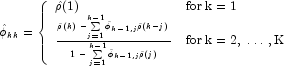
This procedure is sensitive to rounding error and should not be used if the parameters are near the nonstationarity boundary. A possible alternative would be to estimate ${\{\phi_{kk}\}}$ for successive AR(k) models using least or maximum likelihood. Based on the hypothesis that the true process is AR(p), Box and Jenkins (1976, page 65) note

${\rm var}{\{ \hat\phi_{kk}\}} \simeq \frac {1}{n} \;\;\;\;\; {\rm k}\; \geq \; {\rm p + 1}$

See Box and Jenkins (1976, pages 82-84) for more information concerning the partial autocorrelation function.

Requirements

Namespace: Imsl.Stat

Assembly: ImslCS (in ImslCS.dll)

AutoCorrelation Class

Thread Safety

Remarks

Requirements

See Also