Namespace:
Imsl.Stat
Assembly:
ImslCS (in ImslCS.dll) Version: 6.5.0.0
 Syntax
| C# |
|---|
[SerializableAttribute] public class ARMA |
| Visual Basic (Declaration) |
|---|
<SerializableAttribute> _ Public Class ARMA |
| Visual C++ |
|---|
[SerializableAttribute] public ref class ARMA |
Remarks
Class ARMA computes estimates of parameters for a nonseasonal
ARMA model given a sample of observations, ![]() ,
for
,
for ![]() , where n =
z.Length. There are two methods, method of moments and least
squares, from which to choose. The default is method of moments.
, where n =
z.Length. There are two methods, method of moments and least
squares, from which to choose. The default is method of moments.
Two methods of parameter estimation, method of moments and least squares, are provided. The user can choose a method using the Method property. If the user wishes to use the least-squares algorithm, the preliminary estimates are the method of moments estimates by default. Otherwise, the user can input initial estimates by using the SetInitialEstimates method. The following table lists the appropriate methods and properties for both the method of moments and least-squares algorithm:
| Least Squares | Both Method of Moment and Least Squares |
|---|---|
| Center | |
| ARLags | Method |
| MALags | RelativeError |
| Backcasting | MaxIterations |
| ConvergenceTolerance | Mean |
| SetInitialEstimates | Mean |
| Residual | AutoCovariance |
| SSResidual | Variance |
| ParamEstimatesCovariance | Constant |
| AR | |
| MA |
Method of Moments Estimation
Suppose the time series ![]() is generated by an
ARMA (p, q) model of the form
is generated by an
ARMA (p, q) model of the form
Let ![]() be the
estimate of the mean
be the
estimate of the mean ![]() of the time series
of the time series
![]() , where
, where ![]() equals the following:
equals the following:
The autocovariance function is estimated by
for ![]() , where K = p + q.
Note that
, where K = p + q.
Note that ![]() is an estimate of the
sample variance.
is an estimate of the
sample variance.
Given the sample autocovariances, the function computes the method of moments estimates of the autoregressive parameters using the extended Yule-Walker equations as follows:
where
The overall constant ![]() is estimated by the
following:
is estimated by the
following:
The moving average parameters are estimated based on a system of
nonlinear equations given K = p + q + 1 autocovariances,
![]() ,
and p autoregressive parameters
,
and p autoregressive parameters ![]() for
for
![]() .
.
Let ![]() . The autocovariances of the
derived moving average process
. The autocovariances of the
derived moving average process ![]() are estimated by the following relation:
are estimated by the following relation:
The iterative procedure for determining the moving average parameters is based on the relation
where ![]() denotes the autocovariance
function of the original
denotes the autocovariance
function of the original ![]() process.
process.
Let ![]() and
and
![]() , where
, where
and
Then, the value of ![]() at the (i + 1)-th iteration
is determined by the following:
at the (i + 1)-th iteration
is determined by the following:
The estimation procedure begins with the initial value
and terminates at iteration i when either ![]() is less than RelativeError or i
equals MaxIterations. The moving average parameter estimates are
obtained from the final estimate of
is less than RelativeError or i
equals MaxIterations. The moving average parameter estimates are
obtained from the final estimate of ![]() by setting
by setting
The random shock variance is estimated by the following:
See Box and Jenkins (1976, pp. 498-500) for a description of a function that performs similar computations.
Least-squares Estimation
Suppose the time series ![]() is generated by a
nonseasonal ARMA model of the form,
is generated by a
nonseasonal ARMA model of the form,
where B is the backward shift operator, ![]() is the mean of
is the mean of ![]() , and
, and
with p autoregressive and q moving average parameters. Without loss of generality, the following is assumed:
so that the nonseasonal ARMA model is of order ![]() , where
, where ![]() and
and
![]() . Note that the usual hierarchical
model assumes the following:
. Note that the usual hierarchical
model assumes the following:
Consider the sum-of-squares function
where
and T is the backward origin. The random shocks
![]() are assumed to be independent and
identically distributed
are assumed to be independent and
identically distributed
random variables. Hence, the log-likelihood function is given by
where ![]() is a function of
is a function of
![]() .
.
For T = 0, the log-likelihood function is conditional on
the past values of both ![]() and
and
![]() required to initialize the model. The method
of selecting these initial values usually introduces transient bias into
the model (Box and Jenkins 1976, pp. 210-211). For
required to initialize the model. The method
of selecting these initial values usually introduces transient bias into
the model (Box and Jenkins 1976, pp. 210-211). For
![]() , this dependency vanishes, and
estimation problem concerns maximization of the unconditional
log-likelihood function. Box and Jenkins (1976, p. 213) argue that
, this dependency vanishes, and
estimation problem concerns maximization of the unconditional
log-likelihood function. Box and Jenkins (1976, p. 213) argue that
dominates
The parameter estimates that minimize the sum-of-squares function are called least-squares estimates. For large n, the unconditional least-squares estimates are approximately equal to the maximum likelihood-estimates.
In practice, a finite value of T will enable sufficient
approximation of the unconditional sum-of-squares function. The values
of ![]() needed to compute the unconditional sum of
squares are computed iteratively with initial values of
needed to compute the unconditional sum of
squares are computed iteratively with initial values of
![]() obtained by back forecasting. The residuals
(including backcasts), estimate of random shock variance, and covariance
matrix of the final parameter estimates also are computed. ARIMA
parameters can be computed by using Difference with ARMA.
obtained by back forecasting. The residuals
(including backcasts), estimate of random shock variance, and covariance
matrix of the final parameter estimates also are computed. ARIMA
parameters can be computed by using Difference with ARMA.
Forecasting
The Box-Jenkins forecasts and their associated probability limits for a
nonseasonal ARMA model are computed given a sample of n =
z.Length, ![]() for
for
![]() .
.
Suppose the time series ![]() is generated by a
nonseasonal ARMA model of the form
is generated by a
nonseasonal ARMA model of the form
for ![]() ,
where B is the backward shift operator,
,
where B is the backward shift operator,
![]() is the constant, and
is the constant, and
with p autoregressive and q moving average parameters. Without loss of generality, the following is assumed:
so that the nonseasonal ARMA model is of order
![]() , where
, where
![]() and
and
![]() . Note that the usual hierarchical
model assumes the following:
. Note that the usual hierarchical
model assumes the following:
The Box-Jenkins forecast at origin t for lead time l of
![]() is defined in terms of the difference
equation
is defined in terms of the difference
equation
where the following is true:
The ![]() percent probability limits for
percent probability limits for
![]() are given by
are given by
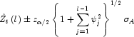
where ![]() is the
is the
![]() percentile of the standard normal
distribution
percentile of the standard normal
distribution
and
are the parameters of the random shock form of the difference equation.
Note that the forecasts are computed for lead times
![]() at origins
at origins
![]() , where
, where
![]() and
and
![]() .
.
The Box-Jenkins forecasts minimize the mean-square error
Also, the forecasts can be easily updated according to the following equation:
This approach and others are discussed in Chapter 5 of Box and Jenkins (1976).