fastPoisson2d¶

Solves Poisson’s or Helmholtz’s equation on a two-dimensional rectangle using a fast Poisson solver based on the HODIE finite-difference scheme on a uniform mesh.

Synopsis¶

fastPoisson2d (rhsPde, rhsBc, coeffU, nx, ny, ax, bx, ay, by, bcType)

Required Arguments¶

float rhsPde (x, y): User-supplied function to evaluate the right-hand side of the partial differential equation at x and y.
float rhsBc(side, x, y): User-supplied function to evaluate the right-hand side of the boundary conditions, on side side, at x and y. The value of side will be one of the following: RIGHT_SIDE, BOTTOM_SIDE, LEFT_SIDE, or TOP_SIDE.
float coeffU (Input): Value of the coefficient of u in the differential equation.
int nx (Input): Number of grid lines in the x-direction. nx must be at least 4. See the Description section for further restrictions on nx.
int ny (Input): Number of grid lines in the y-direction. ny must be at least 4. See the Description section for further restrictions on ny.
float ax (Input): The value of x along the left side of the domain.
float bx (Input): The value of x along the right side of the domain.
float ay (Input): The value of y along the bottom of the domain.
float by (Input): The value of y along the top of the domain.
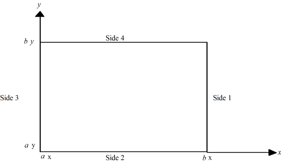
int bcType[4] (Input): Array of size 4 indicating the type of boundary condition on each side of the domain or that the solution is periodic. The sides are numbered as follows:

Side	Location
`RIGHT_SIDE`(0)	x = `bx`
`BOTTOM_SIDE`(1)	y = `ay`
`LEFT_SIDE`(2)	x = `ax`
`TOP_SIDE`(3)	y = `by`
The three possible boundary condition types are as follows:
Type	Location
`DIRICHLET_BC`	Value of u is given.
`NEUMANN_BC`	Value of du/dx is given (on the right or left sides) or du/dy (on the bottom or top of the domain).
`PERIODIC_BC`	Periodic

Return Value¶

An array of size nx by ny containing the solution at the grid points.

Optional Arguments¶

order, int (Input)

Order of accuracy of the finite-difference approximation. It can be either 2 or 4.

Default: order = 4

Description¶

Let c = coeffU, \(a_x\) = ax, \(b_x\) = bx, \(a_y\) = ay, \(b_y\) = by, \(n_x\) = nx and \(n_y\) = ny.

fastPoisson2d is based on the code HFFT2D by Boisvert (1984). It solves the equation

\[\frac{\partial^2 u}{\partial x^2} + \frac{\partial^2 u}{\partial y^2} + cu = p\]

on the rectangular domain \((a_x, b_x) \times (a_y, b_y)\) with a user-specified combination of Dirichlet (solution prescribed), Neumann (first-derivative prescribed), or periodic boundary conditions. The sides are numbered clockwise, starting with the right side.

When \(c = 0\) and only Neumann or periodic boundary conditions are prescribed, then any constant may be added to the solution to obtain another solution to the problem. In this case, the solution of minimum ∞-norm is returned.

The solution is computed using either a second-or fourth-order accurate finite-difference approximation of the continuous equation. The resulting system of linear algebraic equations is solved using fast Fourier transform techniques. The algorithm relies on the fact that \(n_x - 1\) is highly composite (the product of small primes). For details of the algorithm, see Boisvert (1984). If \(n_x - 1\) is highly composite then the execution time of fastPoisson2d is proportional to \(n_x n_y \log_2 n_x\). If evaluations of \(p(x, y)\) are inexpensive, then the difference in running time between order = 2 and order = 4 is small.

The grid spacing is the distance between the (uniformly spaced) grid lines. It is given by the formulas hx = (bx - ax)/(nx -1) and hy = (by - ay)/(ny - 1). The grid spacings in the x and y directions must be the same, i.e., nx and ny must be such that hx is equal to hy. Also, as noted above, nx and ny must be at least 4. To increase the speed of the fast Fourier transform, nx - 1 should be the product of small primes. Good choices are 17, 33, and 65.

If -coeffU is nearly equal to an eigenvalue of the Laplacian with homogeneous boundary conditions, then the computed solution might have large errors.

Example¶

In this example, the equation

\[\frac{\delta^2u}{\delta x_2} + \frac{\delta^2u}{\delta y^2} + 3u = -2 \sin(x + 2y) + 16e^{2x+3y}\]

with the boundary conditions

\[\frac{du}{dy} = 2 \cos(x+2y) + 3e^{2x+3y}\]

on the bottom side and

\[u = \sin(x+2y) + e^{2x+3y}\]

on the other three sides is solved. The domain is the rectangle [0, ¼] ×[0, ½]. The output of fastPoisson2d is a 17 × 33 table of values. The functions spline2dValue are used to print a different table of values.

from __future__ import print_function
from numpy import *
from pyimsl.math.fastPoisson2d import fastPoisson2d, \
    RIGHT_SIDE, BOTTOM_SIDE, LEFT_SIDE, TOP_SIDE, \
    DIRICHLET_BC, NEUMANN_BC
from pyimsl.math.spline2dInterp import spline2dInterp
from pyimsl.math.spline2dValue import spline2dValue


def rhs_pde(x, y):
    # Define the right side of the PDE
    return (-2.0 * sin(x + 2.0 * y) + 16.0 * exp(2.0 * x + 3.0 * y))


def rhs_bc(side, x, y):
    # Define the boundary conditions
    if (side == BOTTOM_SIDE):
        return (2.0 * cos(x + 2.0 * y) + 3.0 * exp(2.0 * x + 3.0 * y))
    else:
        return (sin(x + 2.0 * y) + exp(2.0 * x + 3.0 * y))


nx = 17
nxtabl = 5
ny = 33
nytabl = 5
bc_type = zeros((4), dtype='int')
xdata = zeros((nx), dtype='double')
ydata = zeros((ny), dtype='double')

# Set rectangle size
ax = 0.0
bx = 0.25
ay = 0.0
by = 0.50

# Set boundary conditions
bc_type[RIGHT_SIDE] = DIRICHLET_BC
bc_type[BOTTOM_SIDE] = NEUMANN_BC
bc_type[LEFT_SIDE] = DIRICHLET_BC
bc_type[TOP_SIDE] = DIRICHLET_BC

# Coefficient of u
coefu = 3.0

# Solve the PDE
u = fastPoisson2d(rhs_pde, rhs_bc, coefu, nx, ny, ax, bx, ay, by, bc_type)

# Set up for interpolation
for i in range(0, nx):
    xdata[i] = ax + (bx - ax) * float(i) / float(nx - 1)
for i in range(0, ny):
    ydata[i] = ay + (by - ay) * float(i) / float(ny - 1)

# Compute interpolant
sp = spline2dInterp(xdata, ydata, u)
print("     x          y          u        error")
for i in range(0, nxtabl):
    for j in range(0, nytabl):
        x = ax + (bx - ax) * float(j) / float(nxtabl - 1)
        y = ay + (by - ay) * float(i) / float(nytabl - 1)
        u_table = spline2dValue(x, y, sp)
        abs_error = abs(u_table - sin(x + 2.0 * y)
                        - exp(2.0 * x + 3.0 * y))
        # Print computed answer and absolute on
        # nxtabl by nytabl grid
        print("  %6.4f     %6.4f     %6.4f     %8.2e"
              % (x, y, u_table, abs_error))

Output¶

     x          y          u        error
0000     0.0000     1.0000     0.00e+00
0625     0.0000     1.1956     1.09e-09
1250     0.0000     1.4087     1.50e-09
1875     0.0000     1.6414     1.17e-09
2500     0.0000     1.8961     4.44e-16
0000     0.1250     1.7024     0.00e+00
0625     0.1250     1.9562     1.14e-09
1250     0.1250     2.2345     1.59e-09
1875     0.1250     2.5407     1.23e-09
2500     0.1250     2.8783     0.00e+00
0000     0.2500     2.5964     0.00e+00
0625     0.2500     2.9322     1.47e-09
1250     0.2500     3.3034     2.04e-09
1875     0.2500     3.7148     1.60e-09
2500     0.2500     4.1720     4.44e-16
0000     0.3750     3.7619     4.44e-16
0625     0.3750     4.2164     1.62e-09
1250     0.3750     4.7226     2.23e-09
1875     0.3750     5.2878     1.80e-09
2500     0.3750     5.9199     1.78e-15
0000     0.5000     5.3232     1.78e-15
0625     0.5000     5.9520     8.88e-16
1250     0.5000     6.6569     8.88e-16
1875     0.5000     7.4483     1.78e-15
2500     0.5000     8.3380     5.33e-15

Fatal Errors¶

IMSL_STOP_USER_FCN

Request from user supplied function to stop algorithm.

User flag = “#”.