splineLeastSquares¶

Computes a least-squares spline approximation.

Synopsis¶

splineLeastSquares (xdata, fdata, splineSpaceDim)

Required Arguments¶

float xdata[] (Input): Array with ndata components containing the abscissas of the least-squares problem.
float fdata[] (Input): Array with ndata components containing the ordinates of the least-squares problem.
int splineSpaceDim (Input): The linear dimension of the spline subspace. It should be smaller than ndata and greater than or equal to order (whose default value is 4).

Return Value¶

The structure that represents the spline fit. If a fit cannot be computed, then None is returned.

Optional Arguments¶

sse (Output)

This option places the weighted error sum of squares in the place pointed to by sse.

weights, float[] (Input)

This option requires the user to provide the weights.

Default: all weights equal one.

order, int (Input)

The order of the spline subspace for which the knots are desired. This option is used to communicate the order of the spline subspace.

Default: order = 4, (i.e., cubic splines).

knots, float[] (Input)

This option requires the user to provide the knots. The user must provide a knot sequence of length splineSpaceDim + order.

Default: an appropriate knot sequence is selected. See below for more details.

optimize

This option optimizes the knot locations, by attempting to minimize the least-squares error as a function of the knots. The optimal knots are available in the returned spline structure.

Description¶

Let’s make the identifications

n = ndata

x = xdata

f = fdata

m = splineSpaceDim

k = order

For convenience, we assume that the sequence x is increasing, although the function does not require this.

By default, \(k = 4\), and the knot sequence we select equally distributes the knots through the distinct \(x_i\)’s. In particular, the m + k knots will be generated in \([x_1, x_n]\) with k knots stacked at each of the extreme values. The interior knots will be equally spaced in the interval.

Once knots t and weights w are determined (and assuming that the option optimize is not chosen), then the function computes the spline least-squares fit to the data by minimizing over the linear coefficients \(a_j\)

\[\sum_{i=0}^{n-1} w_i \left[ f_i - \sum_{j=1}^{m} a_jB_j\left(x_i\right) \right]^2\]

where the \(B_j\), \(j = 1, ..., m\) are a (B-spline) basis for the spline subspace.

The optional argument order allows the user to choose the order of the spline fit. The optional argument knots allows user specification of knots. The function splineLeastSquares is based on the routine L2APPR by de Boor (1978, p. 255).

If the option optimize is chosen, then the procedure attempts to find the best placement of knots that will minimize the least-squares error to the given data by a spline of order k with m coefficients. For this problem to make sense, it is necessary that m > k. We then attempt to find the minimum of the functional

\[F(a,t) = \sum_{i=0}^{n-1} w_i \left[ f_i - \sum_{j=0}^{m-1} a_jB_{j,k,t}\left(x_i\right) \right]\]

The technique employed here uses the fact that for a fixed knot sequence t the minimization in a is a linear least-squares problem that can be easily solved. Thus, we can think of our objective function F as a function of just t by setting

\[G(t) = \min_a F(a,t)\]

A Gauss-Seidel (cyclic coordinate) method is then used to reduce the value of the new objective function G. In addition to this local method, there is a global heuristic built into the algorithm that will be useful if the data arise from a smooth function. This heuristic is based on the routine NEWNOT of de Boor (1978, pp. 184 and 258−261).

The initial guess, \(t^g\), for the knot sequence is either provided by the user or is the default. This guess must be a valid knot sequence for splines of order k with

\[t_0^g \leq \ldots \leq t_{k-1}^g \leq x_i \leq t_m^g \leq \ldots \leq t_{m+k-1}^g i=1, \ldots, M\]

with \(t^g\) nondecreasing, and

\[t_i^g < t_{i+k}^g \text{ for } i = 0, \dots, m-1\]

In regard to execution speed, this function can be several orders of magnitude slower than a simple least-squares fit.

The return value for this function is the structure Imsl_d_spline. This structure contains all the information to determine the spline (stored in B-spline form) that is computed by this function. For example, the following code sequence evaluates this spline at x and returns the value in y.

y = splineValue (x, sp)

In the figure below, two cubic splines are fit to

\[\sqrt{|x|}\]

Both splines are cubics with the same splineSpaceDim = 8. The first spline is computed with the default settings, while the second spline is computed by optimizing the knot locations using the keyword optimize.

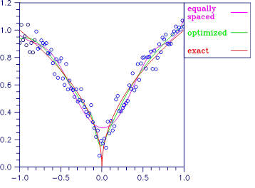
Figure 3.5 — Two Cubic Splines

Examples¶

Example 1¶

This example fits data generated from a trigonometric polynomial

\[1 + sinx + 7 sin3x + ε\]

where ɛ is a random uniform deviate over the range [-1, 1]. The data are obtained by evaluating this function at 90 equally spaced points on the interval [0, 6]. This data is fitted with a cubic spline with 12 degrees of freedom (eight equally spaced interior knots). The error at 10 equally spaced points is printed out.

from __future__ import print_function
from numpy import *
from pyimsl.math.randomSeedSet import randomSeedSet
from pyimsl.math.randomUniform import randomUniform
from pyimsl.math.splineValue import splineValue
from pyimsl.math.splineLeastSquares import splineLeastSquares

# Define function


def F(x):
    return (1. + sin(x) + 7. * sin(3.0 * x))


# Generate random numbers
ndata = 90
spline_space_dim = 12
randomSeedSet(123457)
random = randomUniform(ndata)

# Set up data
xdata = empty(ndata)
fdata = empty(ndata)
for i in range(0, ndata):
    xdata[i] = 6. * i / (ndata - 1)
    fdata[i] = F(xdata[i]) + 2. * (random[i] - .5)
sp = splineLeastSquares(xdata, fdata, spline_space_dim)
print("       x         error")
for i in range(0, 10):
    x = 6. * i / 9.
    error = F(x) - splineValue(x, sp)
    print("%10.3f  %10.3f" % (x, error))

Output¶

       x         error
000      -0.356
667      -0.004
333       0.434
000      -0.069
667      -0.494
333       0.362
000      -0.273
667      -0.247
333       0.303
000       0.578

Example 2¶

This example continues with the first example in which we fit data generated from the trigonometric polynomial

\[1 + sinx + 7 sin3x + ε\]

where ɛ is random uniform deviate over the range [−1, 1]. The data is obtained by evaluating this function at 90 equally spaced points on the interval [0, 6]. This data was fitted with a cubic spline with 12 degrees of freedom (in this case, the default gives us eight equally spaced interior knots) and the error sum of squares was printed. In this example, the knot locations are optimized and the error sum of squares is printed. Then, the error at 10 equally spaced points is printed.

from __future__ import print_function
from numpy import *
from pyimsl.math.randomSeedSet import randomSeedSet
from pyimsl.math.randomUniform import randomUniform
from pyimsl.math.splineValue import splineValue
from pyimsl.math.splineLeastSquares import splineLeastSquares

# Define function


def F(x):
    return (1. + sin(x) + 7. * sin(3.0 * x))


# Generate random numbers
ndata = 90
spline_space_dim = 12
randomSeedSet(123457)
random = randomUniform(ndata)
xdata = empty(ndata)
fdata = empty(ndata)
for delta in range(0, 2):
    for i in range(0, ndata):
        xdata[i] = 6. * i / (ndata - 1)
        fdata[i] = F(xdata[i]) + 2. * (random[i] - .5)
sse1 = []
sp = splineLeastSquares(xdata, fdata, spline_space_dim,
                        sse=sse1)

sse2 = []
sp = splineLeastSquares(xdata, fdata, spline_space_dim,
                        optimize=True,
                        sse=sse2)

print("The error sum of squares before optimizing is %10.1f"
      % (sse1[0]))
print("The error sum of squares  after optimizing is %10.1f"
      % (sse2[0]))
print(" \n      x         Error")
for i in range(0, 10):
    x = 6. * i / 9.
    error = F(x) - splineValue(x, sp)
    print("%10.3f  %10.3f" % (x, error))

Output¶

The error sum of squares before optimizing is       32.6
The error sum of squares  after optimizing is       27.0
 
      x         Error
000      -0.657
667       0.107
333       0.055
000      -0.241
667      -0.064
333      -0.014
000      -0.424
667      -0.139
333       0.134
000       0.495

Warning Errors¶

IMSL_OPT_KNOTS_STACKED_1 The knots found to be optimal are stacked more than order. This indicates fewer knots will produce the same error sum of squares. The knots have been separated slightly.

Fatal Errors¶

`IMSL_XDATA_TOO_LARGE`	The array `xdata` must satisfy \(\text{xdata}_i \leq t_{ndata}\), for i = 1, …, `ndata`.
`IMSL_XDATA_TOO_SMALL`	The array `xdata` must satisfy \(\text{xdata}_i \geq t_{order - 1}\), for i = 1, …, `ndata`.
`IMSL_NEGATIVE_WEIGHTS`	All weights must be greater than or equal to zero.
`IMSL_KNOT_MULTIPLICITY`	Multiplicity of the knots cannot exceed the order of the spline.
`IMSL_KNOT_NOT_INCREASING`	The knots must be nondecreasing.
`IMSL_OPT_KNOTS_STACKED_2`	The knots found to be optimal are stacked more than `order`. This indicates fewer knots will produce the same error sum of squares.