polyRegression¶

Performs a polynomial least-squares regression.

Synopsis¶

polyRegression (xdata, ydata, degree)

Required Arguments¶

float xdata[] (Input): Array of length nObservations containing the independent variable.
float ydata[] (Input): Array of length nObservations containing the dependent variable.
int degree (Input): The degree of the polynomial.

Return Value¶

The vector of size degree +1 containing the coefficients of the fitted polynomial. If a fit cannot be computed, then None is returned.

Optional Arguments¶

weights, float[] (Input): Array with nObservations components containing the vector of weights for the observation. If this option is not specified, all observations have equal weights of one.
ssqPoly (Output): The array containing the sequential sums of squares and other statistics. Row i corresponds to \(x^i\), \(i=1,\ldots,degree\), and the columns are described as follows:

Column	Description
1	degrees of freedom
2	sums of squares
3	F-statistic
4	p-value

ssqLof (Output): The array containing the lack-of-fit statistics. Row i corresponds to \(x^i\), \(i=1,\ldots,degree\), and the columns are described in the following table:

Column	Description
1	degrees of freedom
2	lack-of-fit sums of squares
3	F-statistic for testing lack-of-fit for a polynomial model of degree i
4	p-value for the test

xMean (Output): The mean of x.
xVariance (Output): The variance of x.
anovaTable (Output): The array containing the analysis of variance table.

Element	Analysis of Variance Statistic
0	degrees of freedom for the model
1	degrees of freedom for error
2	total (corrected) degrees of freedom
3	sum of squares for the model
4	sum of squares for error
5	total (corrected) sum of squares
6	model mean square
7	error mean square
8	overall F-statistic
9	p-value
10	\(R^2\) (in percent)
11	adjusted \(R^2\) (in percent)
12	estimate of the standard deviation
13	overall mean of y
14	coefficient of variation (in percent)

dfPureError (Output): If specified, the degrees of freedom for pure error are returned in dfPureError.
ssqPureError (Output): If specified, the sums of squares for pure error are returned in ssqPureError.
residual (Output): The array containing the residuals.

Description¶

The function polyRegression computes estimates of the regression coefficients in a polynomial (curvilinear) regression model. In addition to the computation of the fit, polyRegression computes some summary statistics. Sequential sums of squares attributable to each power of the independent variable (stored in ssqPoly) are computed. These are useful in assessing the importance of the higher order powers in the fit. Draper and Smith (1981, pp. 101-102) and Neter and Wasserman (1974, pp. 278-287) discuss the interpretation of the sequential sums of squares. The statistic \(R^2\) is the percentage of the sum of squares of y about its mean explained by the polynomial curve. Specifically,

\[R^2 = \frac {\Sigma\left(\hat{y}_i-\overline{y}\right)^2} {\Sigma\left(y_1 - \overline{y}\right)^2} 100\%\]

where \(\hat{y}_i\) is the fitted y value at \(x_i\) and \(\bar{y}\) is the mean of y. This statistic is useful in assessing the overall fit of the curve to the data. \(R^2\) must be between 0% and 100%, inclusive. \(R^2\) = 100% indicates a perfect fit to the data.

Estimates of the regression coefficients in a polynomial model are computed using orthogonal polynomials as the regressor variables. This reparameterization of the polynomial model in terms of orthogonal polynomials has the advantage that the loss of accuracy resulting from forming powers of the x-values is avoided. All results are returned to the user for the original model (power form).

The function polyRegression is based on the algorithm of Forsythe (1957). A modification to Forsythe’s algorithm suggested by Shampine (1975) is used for computing the polynomial coefficients. A discussion of Forsythe’s algorithm and Shampine’s modification appears in Kennedy and Gentle (1980, pp. 342-347).

Examples¶

Example 1¶

A polynomial model is fitted to data discussed by Neter and Wasserman (1974, pp. 279-285). The data set contains the response variable y measuring coffee sales (in hundred gallons) and the number of self-service coffee dispensers. Responses for 14 similar cafeterias are in the data set. A graph of the results also is given.

from numpy import *
from pyimsl.math.polyRegression import polyRegression
from pyimsl.math.writeMatrix import writeMatrix

x = array([0.0, 0.0, 1.0, 1.0, 2.0, 2.0, 4.0,
           4.0, 5.0, 5.0, 6.0, 6.0, 7.0, 7.0])
y = array([508.1, 498.4, 568.2, 577.3, 651.7, 657.0, 755.3,
           758.9, 787.6, 792.1, 841.4, 831.8, 854.7, 871.4])
degree = 2

coefficients = polyRegression(x, y, degree)
writeMatrix('Least-Squares Polynomial Coefficients', coefficients,
            rowNumberZero=True, column=True)

Output¶

 
Least-Squares Polynomial Coefficients
           0        503.3
           1         78.9
           2         -4.0

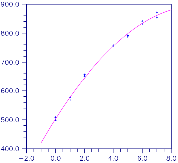
Figure 10.25 — Figure 10-1 A Polynomial Fit

Example 2¶

This example is a continuation of the initial example. Here, many optional arguments are used.

from numpy import *
from pyimsl.math.polyRegression import polyRegression
from pyimsl.math.writeOptions import writeOptions
from pyimsl.math.writeMatrix import writeMatrix

iset = 1
x = array([0.0, 0.0, 1.0, 1.0, 2.0, 2.0, 4.0,
           4.0, 5.0, 5.0, 6.0, 6.0, 7.0, 7.0])
y = array([508.1, 498.4, 568.2, 577.3, 651.7, 657.0, 755.3,
           758.9, 787.6, 792.1, 841.4, 831.8, 854.7, 871.4])
coef_clab = [" ", "intercept", "linear", "quadratic"]
stat_clab = [" ", "Degrees of\nFreedom",
             "Sum of\nSquares", "\nF-Statistic",
             "\np-value"]
anova_rlab = ["degrees of freedom for regression",
              "degrees of freedom for error",
              "total (corrected) degrees of freedom",
              "sum of squares for regression",
              "sum of squares for error",
              "total (corrected) sum of squares",
              "regression mean square",
              "error mean square", "F-statistic",
              "p-value", "R-squared (in percent)",
              "adjusted R-squared (in percent)",
              "est. standard deviation of model error",
              "overall mean of y",
              "coefficient of variation (in percent)"]

degree = 2
sspoly = []
sslof = []
anova = []
sspe = []
dfpe = []
coefficients = polyRegression(x, y, degree,
                              ssqPoly=sspoly,
                              ssqLof=sslof,
                              anovaTable=anova,
                              dfPureError=dfpe,
                              ssqPureError=sspe)
optionValue = iset
writeOptions(-1, optionValue)
writeMatrix("Least-Squares Polynomial Coefficients", coefficients,
            colLabels=coef_clab)
coef_rlab = [coef_clab[2], coef_clab[3]]
writeMatrix("Sequential Statistics", sspoly,
            colLabels=stat_clab,
            rowLabels=coef_rlab,
            writeFormat="%3.1f%8.1f%6.1f%6.4f")
writeMatrix("Lack-of-Fit Statistics", sslof,
            colLabels=stat_clab,
            rowLabels=coef_rlab,
            writeFormat="%3.1f%8.1f%6.1f%6.4f")
writeMatrix("* * * Analysis of Variance * * *\n", anova,
            rowLabels=anova_rlab,
            writeFormat="%9.2f",
            column=True)

Output¶

 
                     Least-Squares Polynomial Coefficients
                        intercept       linear    quadratic
                            503.3         78.9         -4.0
 
                             Sequential Statistics
                        Degrees of    Sum of                      
                           Freedom   Squares  F-Statistic  p-value
             linear            1.0  220644.1       3410.2   0.0000
             quadratic         1.0    4387.7         67.8   0.0000
 
                            Lack-of-Fit Statistics
                        Degrees of    Sum of                      
                           Freedom   Squares  F-Statistic  p-value
             linear            5.0    4794.8         22.0   0.0004
             quadratic         4.0     407.1          2.3   0.1540
 
                       * * * Analysis of Variance * * *

               degrees of freedom for regression            2.00
               degrees of freedom for error                11.00
               total (corrected) degrees of freedom        13.00
               sum of squares for regression           225031.81
               sum of squares for error                   711.70
               total (corrected) sum of squares        225743.51
               regression mean square                  112515.90
               error mean square                           64.70
               F-statistic                               1739.03
               p-value                                      0.00
               R-squared (in percent)                      99.68
               adjusted R-squared (in percent)             99.63
               est. standard deviation of model error       8.04
               overall mean of y                          710.99
               coefficient of variation (in percent)        1.13

Warning Errors¶

`IMSL_CONSTANT_YVALUES`	The y values are constant. A zero-order polynomial is fit. High order coefficients are set to zero.
`IMSL_FEW_DISTINCT_XVALUES`	There are too few distinct x values to fit the desired degree polynomial. High order coefficients are set to zero.
`IMSL_PERFECT_FIT`	A perfect fit was obtained with a polynomial of degree less than `degree`. High order coefficients are set to zero.

Fatal Errors¶

`IMSL_NONNEG_WEIGHT_REQUEST_2`	All weights must be nonnegative.
`IMSL_ALL_OBSERVATIONS_MISSING`	Each (x, y) point contains NaN (not a number). There are no valid data.
`IMSL_CONSTANT_XVALUES`	The x values are constant.