complementaryChiSquaredCdf
Evaluates the complement of the chi-squared cumulative distribution function (CDF).
Synopsis
complementaryChiSquaredCdf (chiSquared, df)
Required Arguments
- float
chiSquared(Input) - Argument for which the complementary chi-squared distribution function is to be evaluated.
- float
df(Input) - Number of degrees of freedom of the complementary chi-squared
distribution.
dfmust be greater than 0.
Return Value
The probability p that a chi-squared random variable takes a value greater
than chiSquared.
Description
Function complementaryChiSquaredCdf evaluates the complement of the CDF,
\(1-F \left( x | \nu\right)\), of a chi-squared random variable x =
chiSquared with ν = df degrees of freedom, where,
is the chi-squared CDF and Γ (⋅) is the gamma function. The value of the complementary chi‑squared CDF at the point x is the probability that the random variable takes a value greater than x.
For \(\nu>v_{max}=1.e7\), complementaryChiSquaredCdf uses the
Wilson-Hilferty approximation (Abramowitz and Stegun [A&S] 1964, Equation
26.4.17) for p in terms of the normal CDF, which is evaluated using
function normalCdf.
For \(v\leq v_{max}\), complementaryChiSquaredCdf uses series
expansions to evaluate p: for \(x<\nu\), complementaryChiSquaredCdf
calculates p using A&S series 6.5.29, and for \(x\geq\nu\),
complementaryChiSquaredCdf calculates p using the continued fraction
expansion of the incomplete gamma function given in A&S equation 6.5.31.
Function complementaryChiSquaredCdf provides higher right tail accuracy
for the complementary chi-squared distribution than does function 1 ‑
chiSquaredCdf.
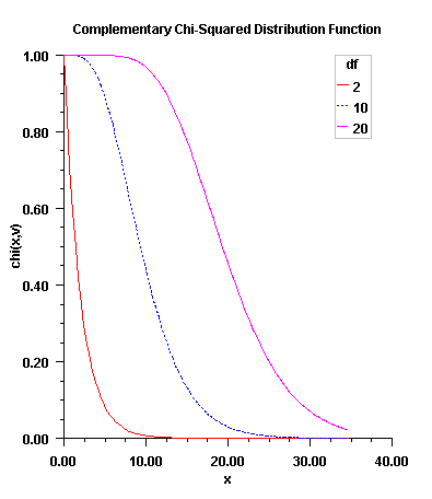
Figure 11.4 — Plot of Fx (x, df)
Example
In this example, we find the probability that X, a chi-squared random variable, is less than 0.15 and the probability that X is greater than 3.0.
from __future__ import print_function
from numpy import *
from pyimsl.stat.chiSquaredCdf import chiSquaredCdf
from pyimsl.stat.complementaryChiSquaredCdf import complementaryChiSquaredCdf

chi_squared = 0.15
df = 2.0

p = chiSquaredCdf(chi_squared, df)
print("The probability that chi-squared")
print(" with df = %1.0f is less than %4.2f is %6.4f" % (df, chi_squared, p))

chi_squared = 3.0
p = complementaryChiSquaredCdf(chi_squared, df)
print(" The probability that chi-squared")
print(" with df = %1.0f is greater than %4.2f is %6.4f" % (df, chi_squared, p))
Output
The probability that chi-squared
 with df = 2 is less than 0.15 is 0.0723
 The probability that chi-squared
 with df = 2 is greater than 3.00 is 0.2231
Informational Errors
IMSLS_COMP_CHISQ_ZERO |
Since “chiSquared” = # is less
than zero, the distribution function is
one at “chiSquared”. |