Introduction to pde_1d_mg
The section describes an algorithm and a corresponding integrator function imsl_f_pde_1d_mg for solving a system of partial differential equations
Equation 1
This software is a one-dimensional differential equation solver. It requires the user to provide initial and boundary conditions in addition to a function for the evaluation of . The integration method is noteworthy due to the maintenance of grid lines in the space variable, . Details for choosing new grid lines are given in Blom and Zegeling, (1994). The class of problems solved with imsl_f_pde_1d_mg is expressed by Equation 1 and given in more detail by:
Equation 2
The vector is the solution. The integer value is the number of differential equations. The functions and can be regarded, in special cases, as flux and source terms. The functions are expected to be continuous. Allowed values for the integer are any of . These are respectively for problems in Cartesian, cylindrical or polar, and spherical coordinates. In the two cases with , the interval must not contain as an interior point.
The boundary conditions have the master equation form
Equation 3
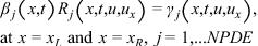
In the boundary conditions the functions and are continuous. In the two cases with , with an endpoint of at 0, the finite value of the solution at must be ensured. This requires the specification of the solution at , or it implies that or . The initial values satisfy , where is a piece-wise continuous vector function of with components.
The user must pose the problem so that mathematical definitions are known for the functions
These functions are provided to the function imsl_f_pde_1d_mg in the form of two user-supplied functions. This form of the usage interface is explained below and illustrated with several examples. can be supplied as the input argument u or by an optional user-supplied function. Users comfortable with the description of this algorithm may skip directly to the Examples section.
Description Summary
Equation 1 is approximated at time-dependent grid values . Using the total differential transforms the differential equation to the form
Using central divided differences for the factor leads to the system of ordinary differential equations in implicit form
The terms respectively represent the approximate solution to the partial differential equation and the value of at the point . The truncation error from this approximation is second-order in the space variable . The above ordinary differential equations are underdetermined, so additional equations are added for determining the time-dependent grid points. These additional equations contain parameters that can be adjusted by the user. Often it will be necessary to modify these parameters to solve a difficult problem. For this purpose the following quantities are needed:
The values are the so-called point concentration of the grid. The parameter denotes a spatial smoothing value. Now the grid points are defined implicitly so that
The parameter denotes a time-smoothing value. If the value is chosen to be large, this results in a fixed spatial grid. Increasing from its default value avoids the error condition where grid lines cross. The divisors are defined by
The value determines the level of clustering or spatial smoothing of the grid points. Decreasing from its default values also decreases the amount of spatial smoothing. The parameters approximate arc length and help determine the shape of the grid or distribution. The parameter prevents the grid movement from adjusting immediately to new values of the , thereby avoiding oscillations in the grid that cause large relative errors in the solution. This is important when applied to solutions with steep gradients.
The discrete form of the differential equation and the smoothing equations are combined to yield the implicit system of differential equations
This is usually a stiff differential-algebraic system. It is solved using the integrator imsl_f_dea_petzold_gear. If imsl_f_dea_petzold_gear is needed during the evaluations of the differential equations or boundary conditions, it must be done in a separate thread to avoid possible problems with imsl_f_pde_1d_mg’s internal use of imsl_f_dea_petzold_gear. The only options for imsl_f_dea_petzold_gear set by imsl_f_pde_1d_mg are the Maximum BDF Order, and the absolute and relative error values, documented as IMSL_MAX_BDF_ORDER, and IMSL_ATOL_RTOL_SCALARS.


