Usage Notes
The functions in this chapter cover a wide variety of commonly used experimental designs. They can be categorized, not only based upon the underlying experimental design that generated the user’s data, but also on whether they provide support for missing values, factorial treatment structure, blocking and replication of the entire experiment, or multiple locations.
Typically, responses are stored in the input vector y. For a few functions, such as imsls_f_anova_oneway and imsls_f_anova_factorial the full set of model subscripts is not needed to identify each response. They assume the usual pattern, which requires that the last model subscript change most rapidly, followed by the model subscript next in line, and so forth, with the first subscript changing at the slowest rate. This pattern is referred to as lexicographical ordering.
However, for most of the functions in this chapter, one or more arrays are used to describe the experimental conditions associated with each value in the response input vector y. The function imsls_f_split_plot, for example, requires three additional input arrays: split, whole and rep. They are used to identify the split-plot, whole-plot and replicate number associated with each value in y.
Many of the functions described in this chapter permit users to enter missing data values using NaN (Not a Number) as the missing value code. Use function imsls_f_machine (or function imsls_d_machine with the double-precision) to retrieve NaN. Any element of y that is missing must be set to imsls_f_machine(6) or imsls_d_machine(6) (for double precision). See imsls_f_machine in Chapter 15, Utilities for a description. Functions imsls_f_anova_factorial, imsls_f_anova_nested and imsls_f_anova_balanced require complete, balanced data, and do not accept missing values.
As a diagnostic tool for validating model assumptions, some functions in this chapter perform a test for lack of fit when replicates are available in each cell of the experimental design.
Completely Randomized Experiments
Completely randomized experiments are analyzed using some variation of the one-way analysis of variance (Anova). A completely randomized design (CRD) is the simplest and most common example of a statistically designed experiment. Researchers using a CRD are interested in comparing the average effect of two or more treatments. In agriculture, treatments might be different plant varieties or fertilizers. In industry, treatments might be different product designs, different manufacturing plants, different methods for delivering the product, etc. In business, different business processes, such as different shipping methods or alternate approaches to a product repair process, might be considered treatments. Regardless of the area, the one thing they have in common is that random errors in the observations cause variations in differences between treatment observations, making it difficult to confirm the effectiveness of one treatment to another.
If observations on these treatments are completely independent then the design is referred to as a completely randomized design or CRD. The IMSL C Numerical Library has two functions for analysis of data from CRD: imsls_f_anova_oneway and imsls_f_crd_factorial.
Both functions allow users to specify observations with missing values, have unequal group sizes, and output treatment means and standard deviations. The primary difference between the functions is that:
1. imsls_f_anova_oneway conducts multiple comparisons of treatment functions; whereas imsls_f_crd_factorial requires users to make a call to imsls_f_multiple_comparisons to compare treatment means.
2. imsls_f_crd_factorial can analyze treatments with a factorial treatment structure; whereas imsls_f_anova_oneway does not analyze factorial structures.
3. imsls_f_crd_factorial can analyze data from CRD experiments that are replicated across several blocks or locations. This can happen when the same experiment is repeated at different times or different locations.
Factorial Experiments
In some cases, treatments are identified by a combination of experimental factors. For example, in an octane study comparing several different gasolines, each gasoline could be developed using a combination of two additives, denoted below in Table 1, as Additive A and Additive B.
Treatment | Additive A | Additive B |
1 | No | No |
2 | Yes | No |
3 | No | Yes |
4 | Yes | Yes |
This is referred to as a 2x2 or 22 factorial experiment. There are 4 treatments involved in this study. One contains no additives, i.e. Treatment 1. Treatment 2 and 3 contain only one of the additives and treatment 4 contains both. A one-way anova, such as found in anova_oneway can analyze these data as four different treatments. Three functions, imsls_f_crd_factorial, imsls_f_rcbd_factorial and imsls_f_anova_factorial will analyze these data exploiting the factorial treatment structure. These functions allow users to answer structural questions about the treatments such as:
1. Are the average effects of the additives statistically significant? This is referred to as the factor main effects.
2. Is there an interaction effect between the additives? That is, is the effectiveness of an additive independent of the other?
Both imsls_f_crd_factorial and imsls_f_rcbd_factorial support analysis of a factorial experiment with missing values and multiple locations. The function imsls_f_anova_factorial does not support analysis of experiments with missing values or experiments replicated over multiple locations. The main difference, as the names imply, between imsls_f_crd_factorial and imsls_f_rcbd_factorial is that imsls_f_crd_factorial assumes that treatments were completely randomized to experimental units. Function imsls_f_rcbd_factorial assumes that treatments are blocked.
Blocking
Blocking is an important technique for reducing the impact of experimental error on the ability of the researcher to evaluate treatment differences. Usually this experimental error is caused by differences in location (spatial differences), differences in time (temporal differences) or differences in experimental units. Researchers refer to these as blocking factors. They are identifiable causes known to cause variation in observations between experimental units.
There are several functions that specifically support blocking in an experiment: imsls_f_rcbd_factorial, imsls_f_lattice, and imsls_f_latin_square. The first two functions, imsls_f_rcbd_factorial and imsls_f_lattice, support blocking on one factor.
A requirement of RCBD experiments is that every block must contain observations on every treatment. However, when the number of treatments ( t ) is greater than the block size ( b ), it is impossible to have every block contain observations on every treatment.
In this case, when t > b, an incomplete block design must be used instead of a RCBD. Lattice designs are a type of incomplete block design in which the number of treatments is equal to the square of an integer such as t = 9, 16, 25, etc. Lattice designs were originally described by Yates (1936). The function imsls_f_lattice supports analysis of data from lattice experiments.
Besides the requirement that , another characteristic of lattice experiments is that blocks be grouped into replicates, where each replicate contains one observation for every treatment. This forces the number of blocks in each replicate to be equal to the number of observations per block. That is, the number of blocks per replicate and the number of observations per block are both equal to .
In addition, the number of replicate groups in Lattice experiments is always less than or equal to k+1. If it is equal to k+1 then the design is referred to as a Balanced Lattice. If it is less than k+1 then the design is referred to as a Partially Balanced Lattice. Tables of these experiments and their analysis are tabulated in Cochran & Cox (1950).
Consider, for example, a 3 × 3 balanced-lattice, i.e., k = 3 and t = 9. Notice that the number of replicates is . And the number of blocks per replicate and block size are both k = 3. The total number of blocks is equal to . For a balanced-lattice, .
Replicate I | Replicate II |
Block 1 (T1, T2, T3) | Block 4 (T1, T4, T7) |
Block 2 (T4, T5, T6) | Block 5 (T2, T5, T8) |
Block 3 (T7, T8, T9) | Block 6 (T3, T6, T9) |
Replicate III | Replicate IV |
Block 1 (T1, T2, T3) | Block 4 (T1, T4, T7) |
Block 2 (T4, T5, T6) | Block 5 (T2, T5, T8) |
Block 3 (T7, T8, T9) | Block 6 (T3, T6, T9) |
The Anova table for a balanced-lattice experiment, takes the form shared with other balanced incomplete block experiments. In these experiments, the error term is divided into two components: the Inter-Block Error and the Intra-Block Error. For single and multiple locations, the general format of the Anova tables for Lattice experiments is illustrated in Table 3 and Table 4.
Source | DF | Sum of Squares | Mean Squares |
|---|---|---|---|
REPLICATES | SSR | MSR | |
TREATMENTS(unadj) | SST | MST | |
TREATMENTS(adj) | SSTa | MSTa | |
BLOCKS(adj) | SSBa | MSBa | |
INTRA-BLOCK ERROR | SSE | MSE | |
TOTAL | SSR | ||
Source | DF | Sum of Squares | Mean Squares |
|---|---|---|---|
LOCATIONS | SSL | MSL | |
REPLICATES WITHIN LOCATIONS | SSR | MSR | |
TREATMENTS(unadj) | SST | MST | |
TREATMENTS(adj) | SSTa | MSTa | |
BLOCKS(adj) | SSB | MSB | |
TOTAL | SSTot | ||
Latin Square designs are very popular in cases where:
1. two blocking factors are involved
2. the two blocking factors do not interact with treatments, and
3. the number of blocks for each factor is equal to the number of treatments.
Consider an octane study involving 4 test vehicles tested in 4 bays with 4 test gasolines. This is a natural arrangement for a Latin square experiment. In this case there are 4 treatments, and two blocking factors, test vehicle and bay, each with 4 levels. The Latin Square for this example would look like the following arrangement.
Test Vehicle | |||||
1 | 2 | 3 | 4 | ||
Test | 1 | A | C | B | D |
2 | D | B | A | C | |
Bay | 3 | C | A | D | B |
4 | B | D | C | A | |
As illustrated above in Table 5, the letters A-D are used to denote the four test gasolines, or treatments. The assignment of each treatment to a particular test vehicle and test bay is described in Table 5. Gasoline A, for example, is tested in the following four vehicle/bay combinations: (1/1), (2/3), (3/2), and (4/4).
Notice that each treatment appears exactly once in every row and column. This balance, together with the assumed absence of interactions between treatments and the two blocking factors is characteristic of a Latin Square.
The corresponding Anova table for these data contains information on the blocking factors as well as treatment differences. Notice that the F-test for one of the two blocking factors, test vehicle, is statistically significant (p = 0.048); whereas the other, test bay, is not statistically significant (p = 0.321).
Some researchers might use this as a basis to remove test bay as a blocking factor. In that case, the design can then be analyzed as a RCBD experiment since every treatment is repeated once and only once in every block, i.e., test vehicle.
Source | Degrees of Freedom | Sum of Squares | Mean Squares | F-Test | p-Value |
|---|---|---|---|---|---|
Test Vehicle | 3 | 1.5825 | 0.5275 | 4.83 | 0.048 |
Test Bay | 3 | 0.0472 | 0.157 | 1.44 | 0.321 |
Gasoline | 3 | 4.247 | 1.416 | 12.97 | 0.005 |
Error | 6 | 0.655 | 0.109 | ||
TOTAL | 15 | 6.9575 | |||
Multiple Locations
It is common for a researcher to repeat an experiment and then conduct an analysis of the data. In agricultural experiments, for example, it is common to repeat an experiment at several different farms. In other cases, a researcher may want to repeat an experiment at a specified frequency, such as week, month or year. If these repeated experiments are independent of one another then we can treat them as multiple locations.
Several of the functions in this chapter allow for multiple locations: imsls_f_crd_factorial, imsls_f_rcbd_factorial, imsls_f_lattice, imsls_f_latin_square, imsls_f_split_plot, imsls_f_split_split_plot, imsls_f_strip_plot, imsls_f_strip_split_plot. All of these functions allow for analysis of experiments replicated at multiple locations. By default they all treat locations as a random factor. Function imsls_f_split_plot also allows users to declare locations as a fixed effect.
Split-Plot Designs – Nesting and Restricted Randomization
Originally, split-plot designs were developed for testing agricultural treatments, such as varieties of wheat, different fertilizers or different insecticides. In these original experiments, growing areas were divided into plots. The major treatment factor, such as wheat variety, was randomly assigned to these plots. However, in addition to testing wheat varieties, they wanted to test another treatment factor such as fertilizer. This could have been done using a CRD or RCBD design. If a CRD design was used then treatment combinations would need to be randomly assigned to plots, such as shown below in Table 7.
CRD | |||
|---|---|---|---|
W3F2 | W1F3 | W4F1 | W2F1 |
W2F3 | W1F1 | W1F3 | W1F2 |
W2F2 | W3F1 | W2F1 | W4F2 |
W3F2 | W1F1 | W2F3 | W1F2 |
W4F1 | W3F2 | W3F2 | W4F3 |
W4F3 | W3F1 | W2F2 | W4F2 |
In the CRD illustration above, any plot could have any combination of wheat variety (W1, W2, W3 or W4) and fertilizer (F1, F2 or F3). There is no restriction on randomization in a CRD. Any of the treatments can appear in any of the 24 plots.
If a RCBD were used, all t=12 treatment combinations would need to be arranged in blocks similar to what is described in Table 8, which places one restriction on randomization.
RCBD | ||||
|---|---|---|---|---|
Block 1 | W3F3 | W1F3 | W4F1 | W4F3 |
W2F3 | W1F1 | W3F2 | W1F2 | |
W2F2 | W3F1 | W2F1 | W4F2 | |
Block 2 | W3F2 | W1F1 | W2F3 | W1F2 |
W4F1 | W1F3 | W3F2 | W4F3 | |
The RCBD arrangement is basically a replicated CRD design with a randomization restriction that treatments are divided into two groups of replicates which are assigned to a block of land. Randomization of treatments only occurs within each block.
At first glance, a split-plot experiment could be mistaken for a RCBD experiment since it is also blocked. The split-plot arrangement with only one replicate for this experiment is illustrated below in Table 9. Notice that it appears as if levels of the fertilizer factor (F1, F2, and F3) are nested within wheat variety (W1, W2, W3 and W4), however that is not the case. Varieties were actually randomly assigned to one of four rows in the field. After randomizing wheat varieties, fertilizer was randomized within wheat variety.
Split-Plot Design | ||||
|---|---|---|---|---|
Block 1 | W2 | W2F1 | W2F3 | W2F2 |
W1 | W1F3 | W1F1 | W1F2 | |
W4 | W4F1 | W4F3 | W4F2 | |
W3 | W3F2 | W3F1 | W3F3 | |
Block 2 | W3 | W3F2 | W3F1 | W3F3 |
W1 | W1F3 | W1F1 | W1F2 | |
W4 | W4F1 | W4F3 | W4F2 | |
W2 | W2F1 | W2F3 | W2F2 | |
The essential distinction between split-plot experiments and completely randomized or randomized complete block experiments is the presence of a second factor that is blocked, or nested, within each level of the first factor. This second factor is referred to as the split-plot factor, and the first is referred to as the whole-plot factor.
Both factors are randomized, but with a restriction on randomization of the second factor, the split-plot factor. Whole plots (wheat variety) are randomly assigned, without restriction to plots, or rows in this example. However, the randomization of split-plots (fertilizer) is restricted. It is restricted to random assignment within whole-plots.
Strip-Plot Designs
Strip-plot experiments look similar to split-plot experiments. In fact they are easily confused, resulting in incorrect statistical analyses. The essential distinction between strip-plot and split-plot experiments is the application of the second factor. In a split-plot experiment, levels of the second factor are nested within the whole-plot factor (see Table 11). In strip-plot experiments, the whole-plot factor is completely crossed with the second factor (see Table 10).
This occurs, for example, when an agricultural field is used as a block and the levels of the whole-plot factor are applied in vertical strips across the entire field. Levels of the second factor are assigned to horizontal strips across the same block.
Whole-Plot Factor | |||||
A2 | A1 | A4 | A3 | ||
Strip Plot | B3 | A2B3 | A1B3 | A4B3 | A3B3 |
B1 | A2B1 | A1B1 | A4B1 | A3B1 | |
B2 | A2B2 | A1B2 | A4B2 | A3B2 | |
Whole-Plot Factor | |||
A2 | A1 | A4 | A3 |
A2B1 | A1B3 | A4B1 | A3B3 |
A2B3 | A1B1 | A4B3 | A3B1 |
A2B2 | A1B2 | A4B2 | A3B2 |
As described in the previous section, in a split-plot experiment the second experimental factor, referred to as the split-plot factor, is nested within the first factor, referred to as the whole-plot factor.
Consider, for example, the semiconductor experiment described in Figure 5, Split-Plot Randomization. The wafers from each plater, the whole-plot factor, are divided into equal size groups and then randomly assigned to an etcher, the split-plot factor. Wafers from different platers are etched separately from those that went through another plating machine. Randomization occurred within each level of the whole-plot factor, i.e., plater.
Graphically, as shown below, this arrangement appears similar to a tree or hierarchical structure.
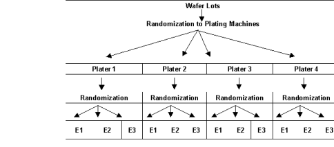
Figure 5, Split-Plot Randomization
Notice that although there are only three etchers, 12 different runs are made using these etchers. The wafers randomly assigned to the first plater and first etcher are processed separately from the wafers assigned to other plating machines.
In a strip-plot experiment, the second randomization of the wafers to etchers occurs differently, see Figure 6, Strip-Plot Semiconductor Experiment. Instead of randomizing the wafers from each plater to the three etchers and then running them separately from the wafers from another plater, the wafers from each plater are divided into three groups and then each randomly assigned to one of the three etchers. However, the wafers from all four plating machines assigned to the same etcher are run together.
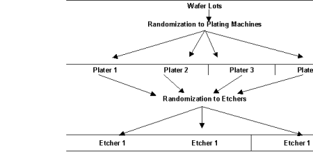
Figure 6, Strip-Plot Semiconductor Experiment
Strip-plot experiments can be analyzed using imsls_f_strip_plot. Function imsls_f_strip_plot returns a strip-plot Anova table with the following general structure:
Source | DF | SS | MS | F-Test | p-Value |
|---|---|---|---|---|---|
Blocks | 1 | 0.0005 | 0.0005 | 0.955 | 0.431 |
Whole-Plots: Plating Machines | 2 | 0.0139 | 0.0070 | 64.39 | 0.015 |
Whole-Plot Error | 2 | 0.0002 | 0.0001 | 0.194 | 0.838 |
Strip-Plots: Etchers | 1 | 0.0033 | 0.0033 | 100.0 | 0.060 |
Strip-Plot Error | 1 | <0.0001 | <0.0001 | 0.060 | 0.830 |
Whole-Plot x Strip-Plot | 2 | 0.0033 | 0.0017 | 2.970 | 0.251 |
Whole-Plot x Strip-Plot Error | 2 | 0.0011 | 0.0006 | ||
TOTAL | 11 | 0.0225 | |||
Split-Split Plot and Strip-Split Plot Experiments
The essential distinction between split-plot and split-split-plot experiments is the presence of a third factor that is blocked, or nested, within each level of the whole-plot and split-plot factors. This third factor is referred to as the sub-plot factor. A split-plot experiment, see Table 13, has only two factors, denoted by A and B. The second factor is nested within the first factor. Randomization of the second factor, the split-plot factor, occurs within each level of the first factor.
Whole-Plot Factor | |||
A2 | A1 | A4 | A3 |
A2B1 | A1B3 | A4B1 | A3B2 |
A2B3 | A1B1 | A4B3 | A3B1 |
A2B2 | A1B2 | A4B2 | A3B3 |
On the other hand, a split-split plot experiment has three factors, illustrated in Table 14 by A, B and C. The second factor is nested within the first factor, and the third factor is nested within the second.
Whole-Plot Factor | |||
A2 | A1 | A4 | A3 |
A2B3C2 A2B3C1 | A1B2C1 A1B2C2 | A4B1C2 A4B1C1 | A3B3C2 A3B3C1 |
A2B1C1 A2B1C2 | A1B1C1 A1B1C2 | A4B3C2 A4B3C1 | A3B2C2 A3B2C1 |
A2B2C2 A2B2C1 | A1B3C1 A1B3C2 | A4B2C1 A4B2C2 | A3B1C2 A3B1C1 |
Contrast the split-split plot experiment to the same experiment run using a strip-split plot design (see Table 15). In a strip-split plot experiment factor B is applied in a strip across factor A; whereas, in a split-split plot experiment, factor B is randomly assigned to each level of factor A. In a strip-split plot experiment, the level of factor B is constant across a row; whereas in a split-split plot experiment, the levels of factor B change as you go across a row, reflecting the fact that for split-plot experiments, factor B is randomized within each level of factor A.
Factor A Strip Plots | |||||
|---|---|---|---|---|---|
A2 | A1 | A4 | A3 | ||
Factor B Strip Plot | B3 | A2B3C2 A2B3C1 | A1B3C1 A1B3C2 | A4B3C2 A4B3C1 | A3B3C2 A3B3C1 |
B1 | A2B1C1 A2B1C2 | A1B1C1 A1B1C2 | A4B1C2 A4B1C1 | A3B1C2 A3B1C1 | |
B2 | A2B2C2 A2B2C1 | A1B2C1 A1B2C2 | A4B2C1 A4B2C2 | A3B2C2 A3B2C1 | |
In some studies, split-split-plot or strip-split-plot experiments are replicated at several locations. Functions imsls_f_split_split_plot and imsls_f_strip_split_plot can analyze these, even when the number of blocks or replicates at each location is different.
Validating Key Assumptions in Anova
The key output in the analysis of designed experiments is the F-tests in the Anova table for that experiment. The validity of these tests relies upon several key assumptions:
1. observational errors are independent of one another,
2. observational errors are Normally distributed, and
3. the variance of observational errors is homogeneous across treatments.
These are referred to as the independence, Normality and homogeneity of variance assumptions. All of these assumptions are evaluated by examining the properties of the residuals, which are estimates of the observational error for each observation. Residuals are calculated by taking the difference between each observed value in the series and its corresponding estimate. In most cases, the residual is the difference between the observed value and the mean for that treatment.
The independence assumption can be examined by evaluating the magnitude of the correlations among the residuals sorted in the order they were collected. The IMSL function imsls_f_autocorrelation (see Chapter 8, Times Series and Forecasting) can be used to obtain these correlations. The autocorrelations, to a maximum lag of about 20, can be examined to identify any that are statistically significant.
Residuals should be independent of one another, which implies that all autocorrelations with a lag of 1 or higher should be statistically equivalent to zero. If a statistically significant autocorrelation is found, leading a researcher to conclude that an autocorrelation is not equal to zero, then this would provide sufficient evidence to conclude that the observational errors are not independent of one another.
The second major assumption for analysis of variance is the Normality assumption. In the IMSL C Numerical Library, functions imsls_f_shapiro_wilk_normality_test, imsls_f_lilliefors_normality_test , and imsls_f_cgi_squared_normality_test (see Chapter 7, Tests of Goodness of Fit) can be used to determine whether the residuals are not Normally distributed. A small p‑value from this test provides sufficient evidence to conclude that the observational errors are not Normally distributed.
The last assumption, homogeneity of variance, is evaluated by comparing treatment standard errors. This is equivalent to testing whether , where is the standard deviation of the observational error for the i‑th treatment. This test can be conducted using imsls_f_homogeneity. To conduct this test, the residuals, and their corresponding treatment identifiers are passed into imsls_f_homogeneity. It calculates the p‑values for both Bartlett’s and Levene’s tests for equal variance. If a p‑value is below the stated significance level, a researcher would conclude that the within treatment variances are not homogeneous.
Multiple Testing
It is well known that the risk of committing a Type I error (i.e., a false positive or false discovery) increases with the number of tests being performed, even if all the tests use the same cut‑off value for significance. The purpose of a multiple testing correction is to control the risk of false positives when performing multiple tests of significance. Two functions are included in this chapter to correct for multiple tests: imsls_f_multiple_comparisons performs multiple comparisons of treatment means using one of four methods to control the overall Type I error rate, and imsls_f_false_discovery_rates calculates false discovery rates and associated q‑values, given a set of p‑values resulting from multiple independent tests.
Missing Observations
Missing observations create problems with the interpretation and calculation of F-tests for designed experiments. The approach taken in the functions described in this chapter is to estimate missing values using the Yates method and then to compute the Anova table using these estimates.
Essentially the Yates method, implemented in imsls_f_yates, replaces missing observations with the values that minimize the error sum of squares in the Anova table. The Anova table is calculated using these estimates, with one modification. The total degrees of freedom and the error degrees of freedom are both reduced by the number of missing observations.
For simple cases, in which only one observation is missing, formulas have been developed for most designs. See Steel and Torrie (1960) and Cochran and Cox (1957) for a description of these formulas. However for more than one missing observation, a multivariate optimization is conducted to simultaneously estimate the missing values. For the simple case with only one missing value, this approach produces estimates identical to the published formulas for a single missing value.
A potential issue arises when the Anova table contains more than one form of error, such as split-plot and strip‑plot designs. In every case, missing values are estimated by minimizing the last error term in the table.


