bayesian_seasonal_adj
Decomposes a time series into trend, seasonal, and an error component.
Synopsis
#include <imsls.h>
float imsls_f_bayesian_seasonal_adj(int nobs, float w[], …, 0)
The type double function is imsls_d_bayesian_seasonal_adj.
Required Arguments
int nobs (Input)
The number of equally spaced series values.
The number of equally spaced series values.
float w[] (Input)
An array of length nobs containing the stationary time series.
An array of length nobs containing the stationary time series.
Return Value
The average Akaike Bayesian Information Criterion for the estimated model. NaN is returned on error.
Synopsis with Optional Arguments
#include <imsls.h>
float imsls_f_bayesian_seasonal_adj (int nobs, float w[],
IMSLS_TREND_ORDER, int t_order,
IMSLS_SEASONAL_ORDER, int s_order,
IMSLS_NUM_PREDICT, int n_predict,
IMSLS_PERIOD, int period,
IMSLS_SPAN, int span,
IMSLS_RIGIDITY, float rigidity,
IMSLS_MODEL, int model,
IMSLS_PRINT_LEVEL, int print_level,
IMSLS_NONSEASONAL_TREND, float **trend,
IMSLS_NONSEASONAL_TREND_USER, float trend[],
IMSLS_SEASONAL, float **seasonal,
IMSLS_SEASONAL_USER, float seasonal[],
IMSLS_IRREGULAR_COMPONENTS, float **irr_comp,
IMSLS_IRREGULAR_COMPONENTS_USER, float irr_comp[],
IMSLS_SERIES_SMOOTHED, float **smoothed,
IMSLS_SERIES_SMOOTHED_USER, float smoothed[],
0)
Optional Arguments
IMSLS_TREND_ORDER, int t_order (Input)
The order of trend differencing where t_order ≥ 0.
Default: t_order = 2.
The order of trend differencing where t_order ≥ 0.
Default: t_order = 2.
IMSLS_SEASONAL_ORDER, int s_order (Input)
The order of seasonal differencing where s_order ≥ 1.
Default: s_order = 1.
The order of seasonal differencing where s_order ≥ 1.
Default: s_order = 1.
IMSLS_NUM_PREDICT, int n_predict (Input)
The number of values to forecast where n_predict ≥ 0.
Default: n_predict = 0.
The number of values to forecast where n_predict ≥ 0.
Default: n_predict = 0.
IMSLS_PERIOD, int period (Input)
The number of seasons within a period where period ≥ 1.
Default: period = 12.
The number of seasons within a period where period ≥ 1.
Default: period = 12.
IMSLS_SPAN, int span (Input)
The number of periods to be processed at one time where 1 ≤ span ≤ nobs/period.
Default: span = nobs/period.
The number of periods to be processed at one time where 1 ≤ span ≤ nobs/period.
Default: span = nobs/period.
IMSLS_RIGIDITY, float rigidity (Input)
Controls the rigidity of the seasonal pattern where 0 ≤ rigidity ≤ 1.0.
Default: rigidity = 1.0.
Controls the rigidity of the seasonal pattern where 0 ≤ rigidity ≤ 1.0.
Default: rigidity = 1.0.
IMSLS_MODEL, int model (Input)
Model option.
Model option.
model | Action |
|---|---|
0 | Non-additive logistic model |
1 | Log additive logistic model |
Default: model = 0.
IMSLS_PRINT_LEVEL, int print_level (Input)
Printing option.
Printing option.
print_level | Action |
|---|---|
0 | No printing |
1 | Prints final results only |
2 | Prints intermediate and final results |
Default: print_level = 0.
IMSLS_NONSEASONAL_TREND, float **trend (Output)
Address of a pointer to an internally allocated array of length nobs + n_predict containing the estimated trend component for each data value followed by the trend estimates for the n_predict forecasted values.
Address of a pointer to an internally allocated array of length nobs + n_predict containing the estimated trend component for each data value followed by the trend estimates for the n_predict forecasted values.
IMSLS_NONSEASONAL_TREND_USER, float trend[] (Output)
Storage array trend is provided by the user. See IMSLS_NONSEASONAL_TREND.
Storage array trend is provided by the user. See IMSLS_NONSEASONAL_TREND.
IMSLS_SEASONAL, float **seasonal (Output)
Address of a pointer to an internally allocated array of length nobs + n_predict containing the estimated seasonal components for each data value followed by the estimates for the n_predict forecasted seasonal values.
Address of a pointer to an internally allocated array of length nobs + n_predict containing the estimated seasonal components for each data value followed by the estimates for the n_predict forecasted seasonal values.
IMSLS_SEASONAL_USER, float seasonal[] (Output)
Storage array seasonal is provided by the user. See IMSLS_SEASONAL above.
Storage array seasonal is provided by the user. See IMSLS_SEASONAL above.
IMSLS_IRREGULAR_COMPONENTS, float **irr_comp (Output)
Address of a pointer to an internally allocated array of length nobs containing the estimated irregular components.
Address of a pointer to an internally allocated array of length nobs containing the estimated irregular components.
IMSLS_IRREGULAR_COMPONENTS_USER, float irr_comp[] (Output)
Storage array irr_comp is provided by the user. See IMSLS_IRREGULAR_COMPONENTS above.
Storage array irr_comp is provided by the user. See IMSLS_IRREGULAR_COMPONENTS above.
IMSLS_SERIES_SMOOTHED, float **smoothed (Output)
Address of a pointer to an internally allocated array of length nobs + n_predict containing the estimated smoothed component for each of the time series values followed by the n_predict forecast values.
Address of a pointer to an internally allocated array of length nobs + n_predict containing the estimated smoothed component for each of the time series values followed by the n_predict forecast values.
IMSLS_SERIES_SMOOTHED_USER, float smoothed[] (Output)
Storage array smoothed is provided by the user. See IMSLS_SERIES_SMOOTHED above.
Storage array smoothed is provided by the user. See IMSLS_SERIES_SMOOTHED above.
Description
Function imsls_f_bayesian_seasonal_adj is based upon the algorithm published by Akaike (1980). This algorithm uses a Bayesian approach to the problem of fitting the following autoregressive model for a time series Wt decomposed into a trend and a seasonal component.
Adopting the notation described earlier in the Usage Notes section of this chapter, if
t ∈ ℤ = {…, -2, - 1, 0, 1, 2, … }
then a seasonal autoregressive model can be represented by the following relationship:
Wt = Tt + St + At
where Wt is the stationary time series with mean μ, Tt denotes an underlying trend, St denotes a seasonal component and At denotes a noise or irregular component.
A non-Bayesian approach to this problem would be to estimate the trend and seasonal components by minimizing
where the difference operator is denoted by ∇ and defined as ∇Tt = (Tt - Tt-1), for k ≥ 1, ∇kTt = ∇(∇k-1Tt), with ∇0Tt = Tt. Similarly, ∇pSt = (St - St-p) and ∇lpSt = ∇p(∇pl-1St), l ≥ 1, with ∇0pSt = St.
The period of the seasonal component, p, the trend order, k, and the seasonal order l correspond to parameter options IMSLS_PERIOD, IMSLS_TREND_ORDER, and IMSLS_SEASONAL_ORDER respectively. d, z, and r are constants determined as follows.
In imsls_f_bayesian_seasonal_adj, the approach is to select the parameter d, which controls the smoothness of the trend and seasonality estimates, using Bayesian methods. The prior distribution controls the smoothness of the trend and seasonal components by assuming low-order Gaussian autoregressive models for some differences of these components. The choice of the variance of the Gaussian distribution is realized by maximizing the log likelihood of the Bayesian model.
The other smoothing parameters, r and z, are determined by the value of rigidity. The default value for rigidity is 1. Larger values of rigidity produce a more rigid seasonal pattern. Normally, a series is first fit using the default value for rigidity. The smoothness of the trend and seasonality estimates are examined and then rigidity is either increased or decreased depending upon whether more or less seasonal smoothing is needed.
Additionally, imsls_f_bayesian_seasonal_adj selects the optimum autoregressive model as the model that minimizes the Akaike Bayesian Information Criterion (ABIC).
ABIC = -2 ln(likelihood)
where the likelihood in this case is the mixed Bayesian maximum likelihood. Smaller values of ABIC represent a better fit. The basic minimization procedure is applied to blocks of data of length span*period. The final return value of the criterion is averaged over these blocks. By default, the data is treated in one block.
Example
This example uses unadjusted unemployment for women over 20 years of age in the U.S. for 1991-2001, as reported by the U.S. Bureau of Labor Statistics (www.bls.gov).
#include <imsls.h>
#include <stdio.h>
#define NDATA 132
#define NFOCAST 12
int main(){
float y[]={2968.0, 3009.0, 2962.0, 2774.0, 3040.0, 3165.0,
3104.0, 3313.0, 3178.0, 3142.0, 3129.0, 3107.0, 3397.0,
3447.0, 3328.0, 3229.0, 3286.0, 3577.0, 3799.0, 3867.0,
3655.0, 3360.0, 3310.0, 3369.0, 3643.0, 3419.0, 3108.0,
3118.0, 3146.0, 3385.0, 3458.0, 3468.0, 3330.0, 3244.0,
3135.0, 3005.0, 3462.0, 3272.0, 3275.0, 2938.0, 2894.0,
3106.0, 3150.0, 3289.0, 3136.0, 2829.0, 2776.0, 2467.0,
2944.0, 2787.0, 2749.0, 2762.0, 2578.0, 2900.0, 3100.0,
3102.0, 2934.0, 2864.0, 2652.0, 2456.0, 3088.0, 2774.0,
2701.0, 2555.0, 2677.0, 2741.0, 3052.0, 2966.0, 2772.0,
2723.0, 2705.0, 2640.0, 2898.0, 2788.0, 2718.0, 2406.0,
2520.0, 2645.0, 2708.0, 2811.0, 2666.0, 2380.0, 2292.0,
2187.0, 2750.0, 2595.0, 2554.0, 2213.0, 2218.0, 2449.0,
2532.0, 2639.0, 2449.0, 2326.0, 2302.0, 2065.0, 2447.0,
2398.0, 2381.0, 2250.0, 2086.0, 2397.0, 2573.0, 2475.0,
2299.0, 2054.0, 2127.0, 1935.0, 2425.0, 2245.0, 2298.0,
2005.0, 2208.0, 2379.0, 2459.0, 2539.0, 2182.0, 1959.0,
2012.0, 1834.0, 2404.0, 2329.0, 2285.0, 2175.0, 2245.0,
2492.0, 2636.0, 2892.0, 2784.0, 2771.0, 2878.0, 2856.0};
int nobs = NDATA, focast = NFOCAST;
float trend[NDATA+NFOCAST], seasonal[NDATA+NFOCAST];
float irr_comp[NDATA], abic=0.0;
char *months[] = {"Jan","Feb","Mar","Apr","May","Jun","Jul",
"Aug","Sep","Oct","Nov","Dec"};
char *years[] = {"","1991","1992","1993","1994","1995",
"1996","1997","1998","1999","2000","2001","2002"};
abic = imsls_f_bayesian_seasonal_adj(nobs, y,
IMSLS_TREND_ORDER, 2,
IMSLS_SEASONAL_ORDER, 1,
IMSLS_NUM_PREDICT, focast,
IMSLS_NONSEASONAL_TREND_USER, &trend,
IMSLS_SEASONAL_USER, &seasonal,
IMSLS_IRREGULAR_COMPONENTS_USER, &irr_comp,
0);
printf("Average ABIC = %f\n", abic);
imsls_f_write_matrix("TREND with last 12 values forecasted",
12, 12, trend,
IMSLS_TRANSPOSE,
IMSLS_ROW_LABELS, months,
IMSLS_COL_LABELS, years,
IMSLS_WRITE_FORMAT, "%8.1f",
0);
imsls_f_write_matrix("SEASONAL with last 12 values forecasted",
12, 12, seasonal,
IMSLS_TRANSPOSE,
IMSLS_ROW_LABELS, months,
IMSLS_COL_LABELS, years,
IMSLS_WRITE_FORMAT, "%6.1f",
0);
imsls_f_write_matrix("IRREGULAR=Original data-TREND-SEASONAL",
11, 12, irr_comp,
IMSLS_TRANSPOSE,
IMSLS_ROW_LABELS, months,
IMSLS_COL_LABELS, years,
IMSLS_WRITE_FORMAT, "%6.1f",
0);
}
Output
Average ABIC = 1297.640259
TREND with last 12 values forecasted
1991 1992 1993 1994 1995 1996 1997
Jan 2879.8 3318.9 3422.6 3228.7 2827.3 2795.7 2743.1
Feb 2918.2 3359.9 3387.8 3206.0 2815.8 2785.6 2720.6
Mar 2955.1 3399.1 3355.5 3177.0 2812.4 2777.9 2694.2
Apr 2990.0 3436.1 3329.5 3142.1 2814.7 2773.2 2665.2
May 3022.7 3469.0 3309.6 3103.9 2819.3 2771.3 2636.0
Jun 3052.8 3496.1 3294.8 3064.8 2825.5 2771.0 2607.4
Jul 3082.8 3514.5 3283.8 3025.7 2830.9 2772.4 2580.8
Aug 3116.2 3521.9 3276.0 2987.3 2833.2 2773.6 2557.2
Sep 3153.4 3517.8 3270.3 2949.0 2831.7 2774.7 2536.3
Oct 3193.8 3503.7 3264.8 2911.3 2826.1 2774.5 2518.0
Nov 3235.6 3482.4 3256.8 2876.6 2816.6 2770.4 2503.0
Dec 3277.6 3455.2 3245.3 2847.6 2805.9 2760.2 2491.5
1998 1999 2000 2001 2002
Jan 2481.3 2352.1 2235.9 2206.0 3166.1
Feb 2469.7 2345.6 2237.6 2239.0 3275.1
Mar 2455.4 2338.1 2239.3 2281.4 3384.1
Apr 2439.0 2328.3 2238.9 2333.1 3493.0
May 2422.8 2315.5 2235.2 2393.9 3602.0
Jun 2408.5 2301.4 2226.3 2464.7 3710.9
Jul 2396.8 2286.0 2212.8 2545.7 3819.9
Aug 2387.7 2269.8 2196.6 2636.7 3928.9
Sep 2380.3 2255.5 2181.3 2735.7 4037.8
Oct 2373.6 2244.6 2171.9 2840.4 4146.8
Nov 2366.6 2238.3 2172.1 2948.2 4255.8
Dec 2359.1 2235.6 2183.3 3057.2 4364.7
SEASONAL with last 12 values forecasted
1991 1992 1993 1994 1995 1996 1997 1998 1999
Jan 162.9 165.6 169.3 172.0 173.8 176.3 176.4 177.3 176.4
Feb 51.4 51.5 50.5 49.5 48.6 48.8 50.0 51.1 51.0
Mar -24.0 -23.9 -23.4 -18.8 -16.3 -13.0 -8.7 -4.9 -3.0
Apr -191.0 -190.1 -189.1 -188.0 -186.6 -187.8 -188.5 -187.9 -186.6
May -140.6 -143.3 -145.4 -147.4 -148.1 -147.1 -147.1 -147.9 -147.7
Jun 67.2 66.6 65.8 64.4 63.3 62.2 62.7 63.6 64.9
Jul 176.9 180.1 181.6 183.0 185.5 186.6 185.8 186.1 187.2
Aug 251.9 253.0 252.6 253.3 253.1 252.8 253.7 254.4 255.2
Sep 76.4 77.2 77.1 77.3 75.5 73.3 72.6 70.7 68.9
Oct -79.5 -80.5 -80.1 -80.8 -81.5 -84.3 -87.6 -90.1 -93.4
Nov -119.8 -120.7 -120.5 -120.2 -120.4 -119.7 -119.7 -118.1 -117.6
Dec -235.7 -237.9 -243.0 -247.9 -250.5 -251.2 -254.2 -256.2 -257.5
2000 2001 2002
Jan 177.2 177.6 177.5
Feb 50.8 51.6 51.5
Mar -1.9 -1.7 -1.8
Apr -187.2 -186.5 -186.6
May -145.7 -145.6 -145.7
Jun 65.6 65.1 65.0
Jul 186.4 184.7 184.7
Aug 256.8 256.9 256.9
Sep 67.3 67.0 67.0
Oct -95.1 -94.6 -94.6
Nov -117.3 -116.6 -116.6
Dec -258.1 -257.1 -257.1
IRREGULAR=Original data-TREND-SEASONAL
1991 1992 1993 1994 1995 1996 1997 1998 1999
Jan -74.7 -87.5 51.1 61.2 -57.1 116.0 -21.5 91.4 -81.5
Feb 39.4 35.6 -19.3 16.5 -77.4 -60.4 17.3 74.2 1.5
Mar 30.9 -47.2 -224.1 116.8 -47.1 -63.9 32.5 103.5 45.9
Apr -25.0 -17.0 -22.5 -16.1 133.9 -30.5 -70.6 -38.0 108.3
May 157.8 -39.7 -18.2 -62.6 -93.1 52.8 31.2 -56.9 -81.9
Jun 45.0 14.3 24.4 -23.1 11.2 -92.1 -25.1 -23.2 30.7
Jul -155.6 104.4 -7.4 -58.6 83.6 93.0 -58.6 -50.9 99.9
Aug -55.0 92.1 -60.6 48.4 15.7 -60.4 0.1 -3.1 -49.9
Sep -51.8 60.0 -17.4 109.6 26.8 -76.0 57.1 -2.1 -25.3
Oct 27.7 -63.3 59.3 -1.5 119.4 32.8 -50.3 42.5 -97.1
Nov 13.2 -51.7 -1.3 19.5 -44.3 54.3 -91.3 53.5 6.3
Dec 65.1 151.7 2.7 -132.8 -99.4 131.0 -50.3 -37.9 -43.1
2000 2001
Jan 11.9 20.4
Feb -43.5 38.4
Mar 60.5 5.3
Apr -46.7 28.5
May 118.5 -3.3
Jun 87.1 -37.7
Jul 59.9 -94.4
Aug 85.6 -1.6
Sep -66.6 -18.7
Oct -117.8 25.3
Nov -42.7 46.4
Dec -91.2 56.0
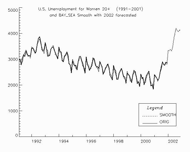
Figure 8, Sample Smoothed Predictions from bayesian_seasonal_adj
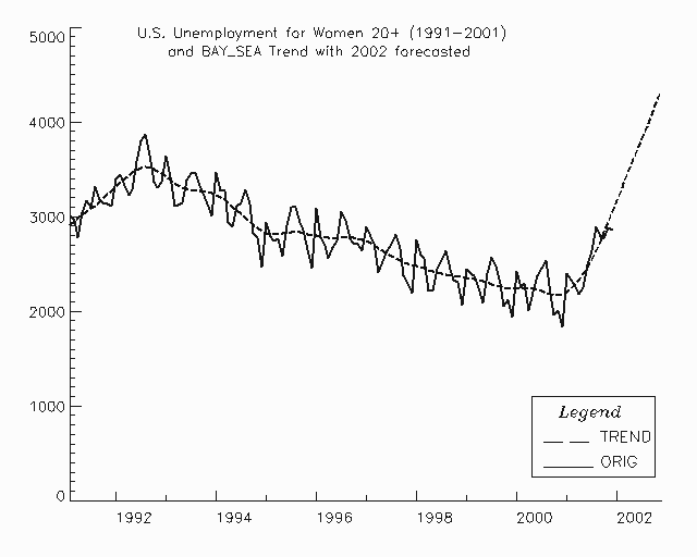
Figure 9, Sample Trend Predictions from bayesian_seasonal_adj


