Section 1.1 describes routines for solving systems of linear algebraic equations by direct matrix factorization methods, for computing only the matrix factorizations, and for computing linear least-squares solutions.

Section 1.2 describes routines for solving systems of parallel constrained least-squares.

Many of the routines described in sections 1.3 and 1.4 are for matrices with special properties or structure. Computer time and storage requirements for solving systems with coefficient matrices of these types can often be drastically reduced, using the appropriate routine, compared with using a routine for solving a general complex system.

The appropriate matrix property and corresponding routine can be located in the “Routines” section. Many of the linear equation solver routines in this chapter are derived from subroutines from LINPACK, Dongarra et al. (1979). Other routines have been developed by Visual Numerics, derived from draft versions of LAPACK subprograms, Bischof et al. (1988), or were obtained from alternate sources.

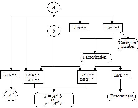
A system of linear equations is represented by Ax = b where A is the n × n coefficient data matrix, b is the known right-hand-side n-vector, and x is the unknown or solution n-vector. Figure 1-1 summarizes the relationships among the subroutines. Routine names are in boxes and input/output data are in ovals. The suffix ** in the subroutine names depend on the matrix type. For example, to compute the determinant of A use LFC** or LFT** followed by LFD**.

The paths using LSA** or LFI** use iterative refinement for a more accurate solution. The path using LSA** is the same as using LFC** followed by LFI**. The path using LSL** is the same as the path using LFC** followed by LFS**. The matrix inversion routines LIN** are available only for certain matrix types.

The two letter codes for the form of coefficient matrix, indicated by ** in Figure 1, are as follows:

The simplest routines to use for solving linear equations are LSL** and LSA**. For example, the mnemonic for matrices of real general form is RG. So, the routines LSARG and LSLRG are appropriate to use for solving linear systems when the coefficient matrix is of real general form. The routine LSARG uses iterative refinement, and more time than LSLRG, to determine a high accuracy solution.

The high accuracy solvers provide maximum protection against extraneous computational errors. They do not protect the results from instability in the mathematical approximation. For a more complete discussion of this and other important topics about solving linear equations, see Rice (1983), Stewart (1973), or Golub and van Loan (1989).

There are situations where the LSL** and LSA** routines are not appropriate. For example, if the linear system has more than one right-hand-side vector, it is most economical to solve the system by first calling a factoring routine and then calling a solver routine that uses the factors. After the coefficient matrix has been factored, the routine LFS** or LFI** can be used to solve for one right-hand side at a time. Routines LFI** uses iterative refinement to determine a high accuracy solution but requires more computer time and storage than routines LFS**.

The routines for evaluating determinants are named LFD**. As indicated in Figure 1-1, these routines require the factors of the matrix as input. The values of determinants are often badly scaled. Additional complications in structures for evaluating them result from this fact. See Rice (1983) for comments on determinant evaluation.

Iterative refinement can often improve the accuracy of a well-posed numerical solution. The iterative refinement algorithm used is as follows:

If the matrix A is in single precision, then the residual ri = Axi-1− b is computed in double precision. If A is in double precision, then quadruple-precision arithmetic routines are used.

The use of the value 50 is arbitrary. In fact a single correction is usually sufficient. It is also helpful even when ri is computed in the same precision as the data.

An inverse of the coefficient matrix can be computed directly by one of the routines named LIN**. These routines are provided for general matrix forms and some special matrix forms. When they do not exist, or when it is desirable to compute a high accuracy inverse, the two-step technique of calling the factoring routine followed by the solver routine can be used. The inverse is the solution of the matrix system AX = I where I denotes the n × n identity matrix, and the solution is X = A-1.

The numerical and mathematical notions of singularity are not the same. A matrix is considered numerically singular if it is sufficiently close to a mathematically singular matrix. If error messages are issued regarding an exact singularity then specific error message level reset actions must be taken to handle the error condition. By default, the routines in this chapter stop. The solvers require that the coefficient matrix be numerically nonsingular. There are some tests to determine if this condition is met. When the matrix is factored, using routines LFC**, the condition number is computed. If the condition number is large compared to the working precision, a warning message is issued and the computations are continued. In this case, the user needs to verify the usability of the output. If the matrix is determined to be mathematically singular, or ill-conditioned, a least-squares routine or the singular value decomposition routine may be used for further analysis.

Toeplitz matrices have entries which are constant along each diagonal, for example:

Real Toeplitz systems can be solved using LSLTO. Complex Toeplitz systems can be solved using LSLTC.

Circulant matrices have the property that each row is obtained by shifting the row above it one place to the right. Entries that are shifted off at the right reenter at the left. For example:

Complex circulant systems can be solved using LSLCC.

The preconditioned conjugate gradient routines PCGRC and JCGRC can be used to solve symmetric positive definite systems. The routines are particularly useful if the system is large and sparse. These routines use reverse communication, so A can be in any storage scheme. For general linear systems, use GMRES.

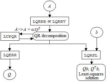
The QR decomposition of a matrix A consists of finding an orthogonal matrix Q, a permutation matrix P, and an upper trapezoidal matrix R with diagonal elements of nonincreasing magnitude, such that AP = QR. This decomposition is determined by the routines LQRRR or LQRRV. It returns R and the information needed to compute Q. To actually compute Q use LQERR. Figure 2 summarizes the relationships among the subroutines.

The QR decomposition can be used to solve the linear system Ax = b. This is equivalent to Rx = QTPb. The routine LQRSL, can be used to find QTPb from the information computed by LQRRR. Then x can be computed by solving a triangular system using LSLRT. If the system Ax = b is overdetermined, then this procedure solves the least-squares problem, i.e., it finds an x for which

is a minimum.

If the matrix A is changed by a rank-1 update, A→A + αxyT, the QR decomposition of A can be updated/down-dated using the routine LUPQR. In some applications a series of linear systems which differ by rank-1 updates must be solved. Computing the QR decomposition once and then updating or down-dating it usually faster than newly solving each system.