FPS2H

Solves Poisson’s or Helmholtz’s equation on a two-dimensional rectangle using a fast Poisson solver based on the HODIE finite-difference scheme on a uniform mesh.
Required Arguments
PRHS — User-supplied FUNCTION to evaluate the right side of the partial differential equation. The form is PRHS(X, Y), where
X – X-coordinate value. (Input)
Y – Y-coordinate value. (Input)
PRHS – Value of the right side at (X, Y). (Output)
PRHS must be declared EXTERNAL in the calling program.
BRHS — User-supplied FUNCTION to evaluate the right side of the boundary conditions. The form is BRHS(ISIDE, X, Y), where
ISIDE – Side number. (Input)
See IBCTY below for the definition of the side numbers.
X - X-coordinate value. (Input)
Y - Y-coordinate value. (Input)
BRHS – Value of the right side of the boundary condition at (X, Y). (Output)
BRHS must be declared EXTERNAL in the calling program.
COEFU — Value of the coefficient of U in the differential equation. (Input)
NX — Number of grid lines in the X-direction. (Input)
NX must be at least 4. See Comment 2 for further restrictions on NX.
NX must be at least 4. See Comment 2 for further restrictions on NX.
NY — Number of grid lines in the Y-direction. (Input)
NY must be at least 4. See Comment 2 for further restrictions on NY.
NY must be at least 4. See Comment 2 for further restrictions on NY.
AX — The value of X along the left side of the domain. (Input)
BX — The value of X along the right side of the domain. (Input)
AY — The value of Y along the bottom of the domain. (Input)
BY — The value of Y along the top of the domain. (Input)
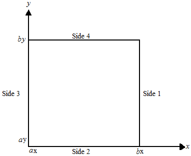
IBCTY — Array of size 4 indicating the type of boundary condition on each side of the domain or that the solution is periodic. (Input)
The sides are numbered 1 to 4 as follows:
The sides are numbered 1 to 4 as follows:
Side | Location |
|---|---|
1 - Right | (X = BX) |
2 - Bottom | (Y = AY) |
3 - Left | (X = AX) |
4 - Top | (Y = BY) |
There are three boundary condition types.
IBCTY | Boundary Condition |
|---|---|
1 | Value of U is given. (Dirichlet) |
2 | Value of dU/dX is given (sides 1 and/or 3). (Neumann) Value of dU/dY is given (sides 2 and/or 4). |
3 | Periodic. |
U — Array of size NX by NY containing the solution at the grid points. (Output)
Optional Arguments
IORDER — Order of accuracy of the finite-difference approximation. (Input)
It can be either 2 or 4. Usually, IORDER = 4 is used.
Default: IORDER = 4.
It can be either 2 or 4. Usually, IORDER = 4 is used.
Default: IORDER = 4.
LDU — Leading dimension of U exactly as specified in the dimension statement of the calling program. (Input)
Default: LDU = size (U,1).
Default: LDU = size (U,1).
FORTRAN 90 Interface
Generic: CALL FPS2H (PRHS, BRHS, COEFU, NX, NY, AX, BX, AY, BY, IBCTY, U [, …])
Specific: The specific interface names are S_FPS2H and D_FPS2H.
FORTRAN 77 Interface
Single: CALL FPS2H (PRHS, BRHS, COEFU, NX, NY, AX, BX, AY, BY, IBCTY, IORDER, U, LDU)
Double: The double precision name is DFPS2H.
Description
Let c = COEFU, ax = AX, bx = BX, ay = AY, by = BY, nx = NX and ny = NY.
FPS2H is based on the code HFFT2D by Boisvert (1984). It solves the equation
on the rectangular domain (ax, bx) × (ay, by) with a user-specified combination of Dirichlet (solution prescribed), Neumann (first-derivative prescribed), or periodic boundary conditions. The sides are numbered clockwise, starting with the right side.
When c = 0 and only Neumann or periodic boundary conditions are prescribed, then any constant may be added to the solution to obtain another solution to the problem. In this case, the solution of minimum ∞‑norm is returned.
The solution is computed using either a second-or fourth-order accurate finite-difference approximation of the continuous equation. The resulting system of linear algebraic equations is solved using fast Fourier transform techniques. The algorithm relies upon the fact that nx ‑ 1 is highly composite (the product of small primes). For details of the algorithm, see Boisvert (1984). If nx ‑ 1 is highly composite then the execution time of FPS2H is proportional to nxny log2 nx. If evaluations of p(x, y) are inexpensive, then the difference in running time between IORDER = 2 and IORDER = 4 is small.
Comments
1. Workspace may be explicitly provided, if desired, by use of F2S2H/DF2S2H. The reference is:
CALL F2S2H (PRHS, BRHS, COEFU, NX, NY, AX, BX, AY, BY, IBCTY, IORDER, U, LDU, UWORK, WORK)
The additional arguments are as follows:
UWORK — Work array of size NX + 2 by NY + 2. If the actual dimensions of U are large enough, then U and UWORK can be the same array.
WORK — Work array of length (NX + 1)(NY + 1)(IORDER ‑ 2)/2 + 6(NX + NY) + NX/2 + 16.
2. The grid spacing is the distance between the (uniformly spaced) grid lines. It is given by the formulas HX = (BX - AX)/(NX - 1) and HY = (BY - AY)/(NY - 1). The grid spacings in the X and Y directions must be the same, i.e., NX and NY must be such that HX equals HY. Also, as noted above, NX and NY must both be at least 4. To increase the speed of the fast Fourier transform, NX - 1 should be the product of small primes. Good choices are 17, 33, and 65.
3. If -COEFU is nearly equal to an eigenvalue of the Laplacian with homogeneous boundary conditions, then the computed solution might have large errors.
Example
In this example, the equation
with the boundary conditions ∂u/∂y = 2 cos(x + 2y) + 3 exp(2x + 3y) on the bottom side and u = sin(x + 2y) + exp(2x + 3y) on the other three sides. The domain is the rectangle [0, 1/4] × [0, 1/2]. The output of FPS2H is a 17 × 33 table of U values. The quadratic interpolation routine QD2VL is used to print a table of values.
USE FPS2H_INT
USE QD2VL_INT
USE UMACH_INT
IMPLICIT NONE
INTEGER NCVAL, NX, NXTABL, NY, NYTABL
PARAMETER (NCVAL=11, NX=17, NXTABL=5, NY=33, NYTABL=5)
!
INTEGER I, IBCTY(4), IORDER, J, NOUT
REAL AX, AY, BRHS, BX, BY, COEFU, ERROR, FLOAT, PRHS, &
TRUE, U(NX,NY), UTABL, X, XDATA(NX), Y, YDATA(NY)
INTRINSIC FLOAT
EXTERNAL BRHS, PRHS
! Set rectangle size
AX = 0.0
BX = 0.25
AY = 0.0
BY = 0.50
! Set boundary condition types
IBCTY(1) = 1
IBCTY(2) = 2
IBCTY(3) = 1
IBCTY(4) = 1
! Coefficient of U
COEFU = 3.0
! Order of the method
IORDER = 4
! Solve the PDE
CALL FPS2H (PRHS, BRHS, COEFU, NX, NY, AX, BX, AY, BY, IBCTY, U)
! Setup for quadratic interpolation
DO 10 I=1, NX
XDATA(I) = AX + (BX-AX)*FLOAT(I-1)/FLOAT(NX-1)
10 CONTINUE
DO 20 J=1, NY
YDATA(J) = AY + (BY-AY)*FLOAT(J-1)/FLOAT(NY-1)
20 CONTINUE
! Print the solution
CALL UMACH (2, NOUT)
WRITE (NOUT,'(8X,A,11X,A,11X,A,8X,A)') 'X', 'Y', 'U', 'Error'
DO 40 J=1, NYTABL
DO 30 I=1, NXTABL
X = AX + (BX-AX)*FLOAT(I-1)/FLOAT(NXTABL-1)
Y = AY + (BY-AY)*FLOAT(J-1)/FLOAT(NYTABL-1)
UTABL = QD2VL(X,Y,XDATA,YDATA,U)
TRUE = SIN(X+2.*Y) + EXP(2.*X+3.*Y)
ERROR = TRUE - UTABL
WRITE (NOUT,'(4F12.4)') X, Y, UTABL, ERROR
30 CONTINUE
40 CONTINUE
END
!
REAL FUNCTION PRHS (X, Y)
REAL X, Y
!
REAL EXP, SIN
INTRINSIC EXP, SIN
! Define right side of the PDE
PRHS = -2.*SIN(X+2.*Y) + 16.*EXP(2.*X+3.*Y)
RETURN
END
!
REAL FUNCTION BRHS (ISIDE, X, Y)
INTEGER ISIDE
REAL X, Y
!
REAL COS, EXP, SIN
INTRINSIC COS, EXP, SIN
! Define the boundary conditions
IF (ISIDE .EQ. 2) THEN
BRHS = 2.*COS(X+2.*Y) + 3.*EXP(2.*X+3.*Y)
ELSE
BRHS = SIN(X+2.*Y) + EXP(2.*X+3.*Y)
END IF
RETURN
END
Output
X Y U Error
0.0000 0.0000 1.0000 0.0000
0.0625 0.0000 1.1956 0.0000
0.1250 0.0000 1.4087 0.0000
0.1875 0.0000 1.6414 0.0000
0.2500 0.0000 1.8961 0.0000
0.0000 0.1250 1.7024 0.0000
0.0625 0.1250 1.9562 0.0000
0.1250 0.1250 2.2345 0.0000
0.1875 0.1250 2.5407 0.0000
0.2500 0.1250 2.8783 0.0000
0.0000 0.2500 2.5964 0.0000
0.0625 0.2500 2.9322 0.0000
0.1250 0.2500 3.3034 0.0000
0.1875 0.2500 3.7148 0.0000
0.2500 0.2500 4.1720 0.0000
0.0000 0.3750 3.7619 0.0000
0.0625 0.3750 4.2163 0.0000
0.1250 0.3750 4.7226 0.0000
0.1875 0.3750 5.2878 0.0000
0.2500 0.3750 5.9199 0.0000
0.0000 0.5000 5.3232 0.0000
0.0625 0.5000 5.9520 0.0000
0.1250 0.5000 6.6569 0.0000
0.1875 0.5000 7.4483 0.0000
0.2500 0.5000 8.3380 0.0000
Published date: 03/19/2020
Last modified date: 03/19/2020


