CHIDF
This function evaluates the chi‑squared cumulative distribution function.
Function Return Value
CHIDF — Function value, the probability that a chi‑squared random variable takes a value less than or equal to CHSQ. (Output)
Required Arguments
CHSQ — Argument for which the chi‑squared distribution function is to be evaluated. (Input)
DF — Number of degrees of freedom of the chi‑squared distribution. (Input)
DF must be positive.
DF must be positive.
Optional Arguments
COMPLEMENT — Logical. If .TRUE., the complement of the chi‑squared cumulative distribution function is evaluated. If .FALSE., the chi‑squared cumulative distribution function is evaluated. (Input)
See the Description section for further details on the use of COMPLEMENT.
Default: COMPLEMENT = .FALSE..
See the Description section for further details on the use of COMPLEMENT.
Default: COMPLEMENT = .FALSE..
FORTRAN 90 Interface
Generic: CHIDF (CHSQ, DF [, …])
Specific: The specific interface names are S_CHIDF and D_CHIDF.
FORTRAN 77 Interface
Single: CHIDF (CHSQ, DF)
Double: The double precision name is DCHIDF.
Description
Function CHIDF evaluates the cumulative distribution function, F, of a chi‑squared random variable with DF degrees of freedom, that is, with ν = DF, and x = CHSQ,
where Γ(⋅) is the gamma function. The value of the distribution function at the point x is the probability that the random variable takes a value less than or equal to x.
For ν > νmax = {343 for double precision, 171 for single precision}, CHIDF uses the Wilson‑Hilferty approximation (Abramowitz and Stegun [A&S] 1964, equation 26.4.17) for p in terms of the normal CDF, which is evaluated using function ANORDF.
For ν ≤ νmax , CHIDF uses series expansions to evaluate p: for x < ν, CHIDF calculates p using A&S series 6.5.29, and for x ≥ ν, CHIDF calculates p using the continued fraction expansion of the incomplete gamma function given in A&S equation 6.5.31.
If COMPLEMENT = .TRUE., the value of CHIDF at the point x is 1 ‑ p, where 1 ‑ p is the probability that the random variable takes a value greater than x. In those situations where the desired end result is 1– p, the user can achieve greater accuracy in the right tail region by using the result returned by CHIDF with the optional argument COMPLEMENT set to .TRUE. rather than by using 1 ‑ p where p is the result returned by CHIDF with COMPLEMENT set to .FALSE..
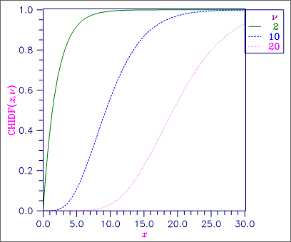
Figure 25, Chi-Squared Distribution Function
Comments
Informational error
Type | Code | Description |
|---|---|---|
1 | 1 | Since the input argument, CHSQ, is less than zero, the distribution function is zero at CHSQ. |
2 | 3 | The normal distribution is used for large degrees of freedom. However, it has produced underflow. Therefore, the probability, CHIDF, is set to zero. |
Example
Suppose X is a chi‑squared random variable with 2 degrees of freedom. In this example, we find the probability that X is less than 0.15 and the probability that X is greater than 3.0.
USE CHIDF_INT
USE UMACH_INT
IMPLICIT NONE
INTEGER NOUT
REAL CHSQ, DF, P
CALL UMACH (2, NOUT)
DF = 2.0
CHSQ = 0.15
P = CHIDF(CHSQ,DF)
WRITE (NOUT,99998) P
99998 FORMAT (' The probability that chi-squared with 2 df is less ', &
'than 0.15 is ', F6.4)
CHSQ = 3.0
P = CHIDF(CHSQ,DF, complement=.true.)
WRITE (NOUT,99999) P
99999 FORMAT (' The probability that chi-squared with 2 df is greater ' &
, 'than 3.0 is ', F6.4)
END
Output
The probability that chi-squared with 2 df is less than 0.15 is 0.0723
The probability that chi-squared with 2 df is greater than 3.0 is 0.2231
Published date: 03/19/2020
Last modified date: 03/19/2020


