DSCRM
Performs a linear or a quadratic discriminant function analysis among several known groups.
Required Arguments
NROW — The absolute value of NROW is the number of rows of X that contain an observation. (Input)
If NROW is negative, the observations are deleted from the discriminant statistics. If NROW is positive, they are added.
If NROW is negative, the observations are deleted from the discriminant statistics. If NROW is positive, they are added.
NVAR — Number of variables to be used in the discrimination. (Input)
X — ∣NROW∣ by NVAR + m matrix containing the data to be used on this call. (Input, if ∣NROW∣ > 0; X is not referenced otherwise)
m is 1, 2, or 3 depending upon whether any columns in X contain frequencies or weights. One column in X must contain the group number for each observation. Group numbers must be 1.0, 2. 0, …, NGROUP. If present, IFRQ gives the column containing the frequencies, while IWT gives the column in X containing the weights.
m is 1, 2, or 3 depending upon whether any columns in X contain frequencies or weights. One column in X must contain the group number for each observation. Group numbers must be 1.0, 2. 0, …, NGROUP. If present, IFRQ gives the column containing the frequencies, while IWT gives the column in X containing the weights.
NGROUP — Number of groups in the data. (Input)
COV — NVAR by NVAR by g matrix of covariances. (Output, for IDO = 0 or 1; input/output, for IDO = 2, 3, or 5; input, for IDO = 4; not referenced if IDO = 6)
g = NGROUP + 1 when IMTH = 1, 2, 4, or 5, and g = 1 otherwise. When IMTH = 3 or 6, the within‑group covariance matrices are not computed. Regardless of the value of IMTH, the pooled covariance matrix is always computed and saved as the g‑th covariance matrix in COV.
g = NGROUP + 1 when IMTH = 1, 2, 4, or 5, and g = 1 otherwise. When IMTH = 3 or 6, the within‑group covariance matrices are not computed. Regardless of the value of IMTH, the pooled covariance matrix is always computed and saved as the g‑th covariance matrix in COV.
COEF — NGROUP by NVAR + 1 matrix containing the linear discriminant function coefficients. (Output, if IDO = 0 or 3; input, if IDO = 4; not referenced if IDO = 1, 2, 5, or 6)
The first column of COEF contains the constant term, and the remaining columns contain the variable coefficients. Row i of COEF corresponds to group i, for i = 1,…,NGROUP. Matrix COEF is always computed as the linear discriminant function coefficients even when quadratic discrimination is specified. Specifically, given the linear discriminant function , the intercept is assigned to COEF(i,1) and the coefficient vector is assigned to COEF(i,2:NVAR+1)for i = 1,…,NGROUP. Matrix COEF is updated if IDO is equal to 0 or 3.
The first column of COEF contains the constant term, and the remaining columns contain the variable coefficients. Row i of COEF corresponds to group i, for i = 1,…,NGROUP. Matrix COEF is always computed as the linear discriminant function coefficients even when quadratic discrimination is specified. Specifically, given the linear discriminant function , the intercept is assigned to COEF(i,1) and the coefficient vector is assigned to COEF(i,2:NVAR+1)for i = 1,…,NGROUP. Matrix COEF is updated if IDO is equal to 0 or 3.
ICLASS — Vector of length ∣NROW∣ containing the group to which the observation was classified. (Output, if IDO = 0 or 4; not referenced otherwise)
If an observation has an invalid group number, frequency, or weight when the leaving‑out‑one method has been specified, then the observation is not classified and the corresponding elements of ICLASS and PROB are set to zero.
If an observation has an invalid group number, frequency, or weight when the leaving‑out‑one method has been specified, then the observation is not classified and the corresponding elements of ICLASS and PROB are set to zero.
PROB — ∣NROW∣ by NGROUP matrix containing the posterior probabilities for each observation. (Output, if IDO = 0 or 4; not referenced otherwise)
CLASS — NGROUP by NGROUP matrix containing the classification table. (Output, if
IDO = 0 or 1, input/output, if IDO = 4; not referenced otherwise)
Each observation that is classified and has a group number equal to 1.0, 2.0, …, NGROUP is entered into the table. The rows of the table correspond to the known group membership. The columns refer to the group to which the observation was classified. Classification results accumulate with each call to DSCRM with IDO = 4. For example, if 2 calls with IDO = 4 are made, then the elements in CLASS sum to the total number of valid observations in the 2 calls.
D2 — NGROUP by NGROUP matrix containing the Mahalanobis distances
between the group means. (Output, when IDO= 0 or 3; not referenced otherwise)
For linear discrimination, the Mahalanobis distance is computed using the pooled covariance matrix. Otherwise, the Mahalanobis distance
For linear discrimination, the Mahalanobis distance is computed using the pooled covariance matrix. Otherwise, the Mahalanobis distance
between group means i and j is computed using the within covariance matrix for group i in place of the pooled covariance matrix.
STAT — Vector of length 4 + 2 * (NGROUP + 1) containing statistics of interest. (Input/ Output, if IDO = 3 or 5; output, if IDO = 0 or 1; not referenced otherwise)
The first element of STAT is the sum of the degrees of freedom for the within‑covariance matrices. The second, third and fourth elements of STAT correspond to the chi‑squared statistic, its degrees of freedom, and the probability of a greater chi‑squared, respectively, of a test of the homogeneity of the within‑covariance matrices (not computed if IMTH = 3 or 6). The 5‑th through 5 + NGROUP elements of STAT contain the log of the determinants of each group’s covariance matrix (not computed if IMTH = 3 or 6) and of the pooled covariance matrix (element 5 + NGROUP). Finally, the last NGROUP + 1 elements of STAT contain the sum of the weights within each group and, in the last position, the sum of the weights in all groups.
The first element of STAT is the sum of the degrees of freedom for the within‑covariance matrices. The second, third and fourth elements of STAT correspond to the chi‑squared statistic, its degrees of freedom, and the probability of a greater chi‑squared, respectively, of a test of the homogeneity of the within‑covariance matrices (not computed if IMTH = 3 or 6). The 5‑th through 5 + NGROUP elements of STAT contain the log of the determinants of each group’s covariance matrix (not computed if IMTH = 3 or 6) and of the pooled covariance matrix (element 5 + NGROUP). Finally, the last NGROUP + 1 elements of STAT contain the sum of the weights within each group and, in the last position, the sum of the weights in all groups.
Optional Arguments
IDO — Processing option. (Input)
Default: IDO = 0.
Default: IDO = 0.
IDO | Action |
|---|---|
0 | This is the only invocation of DSCRM; all the data are input at once. |
1 | This is the first invocation of DSCRM with this data, additional calls will be made. Initialization and updating for the NROW observations are performed. |
2 | This is an intermediate invocation of DSCRM; updating for the NROW observations is performed. |
3 | All statistics are updated for the NROW observations. The discriminant functions and other statistics are computed. |
4 | The discriminant functions are used to classify each of the NROW observations in X. |
5 | The covariance matrices are computed, and workspace is released. No further calls to DSCRM with IDO greater than 1 should be made without first calling DSCRM with IDO = 1. |
6 | Workspace is released. No further calls to DSCRM with IDO greater than 1 should be made without first calling DSCRM with IDO = 1. This option is not required if a call has been made with IDO = 5 or if workspace is explicitly provided by use of D2CRM. |
See Comments 5 and 6 for further information.
NCOL — Number of columns in matrix X. (Input)
Default: NCOL = size (X,2).
Default: NCOL = size (X,2).
LDX — Leading dimension of X exactly as specified in the dimension statement in the calling program. (Input)
Default: LDX = size (X,1).
Default: LDX = size (X,1).
IND — Vector of length NVAR containing the column numbers in X to be used in the discrimination. (Input)
By default, IND(I)=I.
By default, IND(I)=I.
IFRQ — Frequency option. (Input)
IFRQ = 0 means that all frequencies are 1.0. Positive IFRQ indicates that column number IFRQ of X contains the frequencies. All frequencies should be integer values. If this is not the case, the NINT (nearest integer) function is used to obtain integer frequencies.
Default: IFRQ = 0.
IFRQ = 0 means that all frequencies are 1.0. Positive IFRQ indicates that column number IFRQ of X contains the frequencies. All frequencies should be integer values. If this is not the case, the NINT (nearest integer) function is used to obtain integer frequencies.
Default: IFRQ = 0.
IWT — Weighting option. (Input)
IWT = 0 means that all weights are 1.0. Positive IWT means that column IWT of X contains the weights. Negative weights are not allowed.
Default: IWT = 0.
IWT = 0 means that all weights are 1.0. Positive IWT means that column IWT of X contains the weights. Negative weights are not allowed.
Default: IWT = 0.
IGRP — Column number in X containing the group numbers. (Input)
The group numbers must be 1.0, 2,0, …, NGROUP for an observation to be used in the discriminant functions. An observation will be classified regardless of its group number when the reclassification method is specified.
Default: IGRP = NVAR + 1.
The group numbers must be 1.0, 2,0, …, NGROUP for an observation to be used in the discriminant functions. An observation will be classified regardless of its group number when the reclassification method is specified.
Default: IGRP = NVAR + 1.
IMTH — Option parameter giving the method of discrimination. (Input)
IMTH determines whether linear or quadratic discrimination is used whether the group covariance matrices are computed (the pooled covariance matrix is always computed) and whether the leaving‑out‑one or the reclassification method is used to classify each observation.
Default: IMTH = 1.
IMTH determines whether linear or quadratic discrimination is used whether the group covariance matrices are computed (the pooled covariance matrix is always computed) and whether the leaving‑out‑one or the reclassification method is used to classify each observation.
Default: IMTH = 1.
IMTH | Discrim. | Coveriance | Classification |
|---|---|---|---|
1 | Linear | All | Reclassification |
2 | Quadratic | All | Reclassification |
3 | Linear | Pooled only | Reclassification |
4 | Linear | All | Leaving‑out‑one |
5 | Quadratic | All | Leaving‑out‑one |
6 | Linear | Pooled only | Leaving‑out‑one |
In the leaving‑out‑one method of classification, the posterior probabilities are adjusted so as to eliminate the effect of the observation from the sample statistics prior to its classification. In the reclassification method, the effect of the observation is not eliminated from the classification function. Calls to DSCRM with IMTH = 1, 2, 4, or 5 can be intermixed, as can calls to DSCRM with IMTH = 3 or 6. Calls to DSCRM with IMTH = 1, 2, 4, or 5 cannot be intermixed with calls to DSCRM with IMTH = 3 or 6 without first calling DSCRM with IDO = 1 (or 0).
IPRINT — Printing option. (Input)
Default: IPRINT = 0.
For the given combination of IDO and IPRINT, the following arrays are printed.
Default: IPRINT = 0.
For the given combination of IDO and IPRINT, the following arrays are printed.
IPRINT | IDO | Printing |
|---|---|---|
0 | Any | None |
1 or 2 | 0 | PRIOR, NI, XMEAN, COV, COEF, ICLASS, PROB, CLASS, D2, STAT, NRMISS |
1 or 2 | 1 or 2 | None |
1 or 2 | 3 | PRIOR, NI, XMEAN, COEF, D2, STAT, NRMISS |
1 | 4 | None |
2 | 4 | ICLASS, PROB |
1 or 2 | 5 | COV, CLASS |
1 or 2 | 6 | None |
Note that the only change from IPRINT = 1 to IPRINT = 2 is the printing when IDO = 4. Also, note that PRIOR is printed even though it may be input only.
PRIOR — Vector of length NGROUP containing the prior probabilities for each group. (Input, if PRIOR(1) is not ‑1.0 and IDO is 0, 3 or 4; input/output, if PRIOR(1) is ‑1.0 and IDO is 0 or 3; not referenced if IDO is 1, 2, 5 or 6)
If PRIOR(1) is not ‑1.0, then the elements of PRIOR should sum to 1.0. Proportional priors can be selected by setting PRIOR(1) = ‑1.0. In this case, the prior probabilities will be proportional to the sample size in each group, and the elements of PRIOR will contain the proportional prior probabilities after the first call with IDO = 0 or 3. Use of this optional argument is mandatory if IDO = 4.
Default: PRIOR(1) = ‑1.0.
NI — Vector of length NGROUP. (Input, for IDO = 4 or 5; input/output, for IDO = 1, 2 or 3; output, for IDO = 0; not referenced if IDO = 6)
The i‑th element of NI contains the number of observations in group i.
Use of this optional argument is mandatory if IDO = 1, 2, 3, 4, 5.
The i‑th element of NI contains the number of observations in group i.
Use of this optional argument is mandatory if IDO = 1, 2, 3, 4, 5.
XMEAN — NGROUP by NVAR matrix. (Input, for IDO = 3, 4; input/output, for IDO = 2, 5; output, for IDO = 0 or 1; not referenced if IDO = 6)
The i‑th row of XMEAN contains the group i variable means.
The i‑th row of XMEAN contains the group i variable means.
Note that for IDO = 1, 2, 3 ,4 the input and/or output values are just the weighted sums of the observations in each group, i.e. the group i variable means is calculated as
where Mi denotes the number of elements in group i and xik is the k-th observation in group i with associated weight wik and frequency fik.
For IDO = 0 or 5, the means are output and group-wise calculated as weighted arithmetic means,
Use of this optional argument is mandatory if IDO = 1,2,3,4,5.
LDXMEA — Leading dimension of XMEAN exactly as specified in the dimension statement in the calling program. (Input)
Default: LDXMEA = size(XMEAN,1).
Default: LDXMEA = size(XMEAN,1).
LDCOV — Leading and second dimensions of COV exactly as specified in the dimension statement of the calling program. (Input)
The first two dimensions of COV must be equal.
Default: LDCOV = size (COV,1).
The first two dimensions of COV must be equal.
Default: LDCOV = size (COV,1).
LDCOEF — Leading dimension of COEF exactly as specified in the dimension statement in the calling program. (Input)
Default: LDCOEF = size (COEF,1).
Default: LDCOEF = size (COEF,1).
LDPROB — Leading dimension of PROB exactly as specified in the dimension statement in the calling program. (Input)
Default: LDPROB = size (PROB,1).
Default: LDPROB = size (PROB,1).
LDCLAS — Leading dimension of CLASS exactly as specified in the dimension statement in the calling program. (Input)
Default: LDCLAS = size (CLASS,1).
Default: LDCLAS = size (CLASS,1).
LDD2 — Leading dimension of D2 exactly as specified in the dimension statement of the calling program. (Input)
Default: LDD2 = size (D2,1).
Default: LDD2 = size (D2,1).
NRMISS — Number of rows of data encountered in calls to DSCRM containing missing values (NaN) for the classification, group, weight, and/or frequency variables. (Output, if IDO = 0 or 1; input/output, if IDO = 2 or 3, not referenced otherwise)
If a row of data contains a missing value (NaN) for any of these variables, that row is excluded from the computations.
If a row of data contains a missing value (NaN) for any of these variables, that row is excluded from the computations.
FORTRAN 90 Interface
Generic: CALL DSCRM (NROW, NVAR, X, NGROUP, COV, COEF, ICLASS, PROB, CLASS, D2, STAT [, …])
Specific: The specific interface names are S_DSCRM and D_DSCRM.
FORTRAN 77 Interface
Single: CALL DSCRM (IDO, NROW, NVAR, NCOL, X, LDX, IND, IFRQ, IWT, IGRP, NGROUP, IMTH, IPRINT, PRIOR, NI, XMEAN, LDXMEA, COV, LDCOV, COEF, LDCOEF, ICLASS, PROB, LDPROB, CLASS, LDCLAS, D2, LDD2, STAT, NRMISS)
Double: The double precision name is DDSCRM.
Description
Routine DSCRM performs discriminant function analysis using either linear or quadratic discrimination. The output from DSCRM includes a measure of distance between the groups, a table summarizing the classification results, a matrix containing the posterior probabilities of group membership for each observation, and the within‑sample means and covariance matrices. The linear discriminant function coefficients are also computed.
All observations can be input during one call to DSCRM, a method of operation that has the advantage of simplicity. Alternatively, one or more rows of observations can be input during separate calls. This method does not require that all observations be memory resident, a significant advantage with large data sets. Note, however, that DSCRM requires two passes of the data. During the first pass the discriminant functions are computed while in the second pass, the observations are classified. Thus, with the second method of operation, the data will usually need to be input into DSCRM twice.
Because both methods result in the same operations being performed, the algorithm for DSCRM is discussed as if only a few observations are input during each call. The operations performed during each call to DSCRM depend upon the IDO parameter. IDO = 0 should be used if all observations are to be input at one time.
The IDO = 1 step is the initialization step. The variables XMEAN, CLASS, and COV are initialized to zero, and other program parameters are set. After this call, all subroutine arguments except IDO, NROW, X, LDX and IMTH should not be changed by the user except via another call to DSCRM with IDO = 0 or IDO = 1. IMTH can be changed from one call to the next within the two sets {1, 2, 4, 5} or {3, 6} but not between these sets when IDO > 1. That is, do not call DSCRM with IMTH = 1 in one call and IMTH = 3 in another call without first calling DSCRM with IDO = 1.
After initialization has been performed in the IDO = 1 step, the within‑group means are updated for all valid observations in X. Observations with invalid group numbers are ignored, as are observations with missing values. The LU factorization of the covariance matrices are updated by adding (or deleting) observations via Givens rotations.
The IDO = 2 step is used solely for adding or deleting observations from the model as in the above paragraph.
The IDO = 3 step begins by adding all observations in X to the means and the factorizations of the covariance matrices. It continues by computing some statistics of interest: the linear discriminant functions, the prior probabilities (if PRIOR(1) = ‑1.0), the log of the determinant of each of the covariance matrices, a test statistic for testing that all of the within‑group covariance matrices are equal, and a matrix of Mahalanobis distances between the groups. The matrix of Mahalanobis distances is computed via the pooled covariance matrix when linear discrimination is specified, the row covariance matrix is used when the discrimination is quadratic.
Covariance matrices are defined as follows. Let Ni denote the sum of the frequencies of the observations in group i, and let Mi denote the number of observations in group i. Then, if Si denotes the within‑group i covariance matrix,
where wj is the weight of the j-th observation in group i, fj is its frequency, xj is the j-th observation column vector (in group i), and denotes the mean vector of the observations in group i. The mean vectors are computed as
where
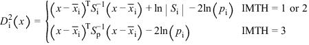
Given the means and the covariance matrices, the linear discriminant function for group i is computed as:
where ln(pi) is the natural log of the prior probability for the i‑th group, x is the observation to be classified, and Sp denotes the pooled covariance matrix.
Let S denote either the pooled covariance matrix or one of the within‑group covariance matrices Si. (S will be the pooled covariance matrix in linear discrimination, and Si otherwise.) The Mahalanobis distance between group i and group j is computed as:
Finally, the asymptotic chi‑squared test for the equality of covariance matrices is computed as follows (Morrison 1976, page 252):
where ni is the number of degrees of freedom in the i‑th sample covariance matrix, k is the number of groups, and
where p is the number of variables.
When IDO = 4, the estimated posterior probability of each observation x belonging to group i is computed using the prior probabilities and the sample mean vectors and estimated covariance matrices under a multivariate normal assumption. Under quadratic discrimination, the within‑group covariance matrices are used to compute the estimated posterior probabilities. The estimated posterior probability of an observation x belonging to group i is
where
For the leaving‑out‑one method of classification (IMTH = 4, 5, and 6), the sample mean vector and sample covariance matrices in the formula for
are adjusted so as to remove the observation x from their computation. For linear discrimination (IMTH = 1, 2, 4, and 6), the linear discriminant function coefficients are actually used to compute the same posterior probabilities.
Using the posterior probabilities, each observations in X is classified into a group; the result is tabulated in the matrix CLASS and saved in the vector ICLASS. CLASS is not altered at this stage if X(i, IGRP) contains a group number that is out of range. If the reclassification method is specified, then all observations with no missing values in the NVAR classification variables are classified. When the leaving‑out‑one method is used, observations with invalid group numbers, weights, frequencies or classification variables are not classified. Regardless of the frequency, a 1 is added (or subtracted) from CLASS for each row of X that is classified and contains a valid group number.
When IMTH > 3, adjustment is made to the posterior probabilities to remove the effect of the observation in the classification rule. In this adjustment, each observation is presumed to have a weight of X(i, IWT), if IWT > 0 and a frequency of 1.0. See Lachenbruch (1975, page 36) for the required adjustment.
Note that the X data in an IDO = 3 call do not have to be identical with the X data used in a subsequent IDO = 4 call if the reclassification method (IMTH=1,2,3) is used: The observations in the IDO = 3 call serve as a training sample to determine the discriminant functions that can be used in the following IDO = 4 call to classify new X data. Since the reclassification method classifies each observation regardless of its group number, it can also be used for the classification of new observations whose actual group assignment is not known (i.e. group column (IGRP) of X is not used when IDO = 4). See Example 3.
Finally, when IDO = 5, the covariance matrices are computed from their LU factorizations, and the mean values (XMEAN) are scaled.
Comments
1. Workspace may be explicitly provided, if desired, by use of D2CRM/DD2CRM. The reference is:
CALL D2CRM (IDO, NROW, NVAR, NCOL, X, LDX, IND, IFRQ, IWT, IGRP, NGROUP, IMTH, IPRINT, RIOR, NI, XMEAN, LDXMEA, COV, LDCOV, COEF, LDCOEF, ICLASS, PROB, LDPROB, CLASS, LDCLAS, D2, LDD2, STAT, NRMISS, D, OB, OB1)
The additional arguments are as follows:
D — Work vector of length equal to (NGROUP + 1) * NVAR if IMTH is not 3 or 6, and of length NVAR otherwise.
OB — Work vector of length equal to NVAR.
OB1 — Work vector of length equal to NVAR.
2. Informational errors
Type | Code | Description |
|---|---|---|
3 | 1 | A row of the data matrix X has an invalid group number. |
4 | 2 | The variance‑covariance matrix for a group is singular. |
4 | 3 | The pooled variance‑covariance matrix is singular. |
3 | 4 | The variance‑covariance matrix for a group is singular. STAT(2) cannot be computed. STAT(2) and STAT(4) are set to the missing value code (NaN). |
3 | 5 | An element of PRIOR is less than or equal to 10−20. |
3 | 6 | The leaving‑out‑one method is specified, but this observation does not have a valid weight, or it does not have a valid frequency. This observation is ignored. |
3 | 7 | The leaving‑out‑one method is specified, but this observation does not have a valid group number. This observation is ignored. |
3. Common choices for the Bayesian prior probabilities are given by:
PRIOR(i) = 1.0/NGROUP (equal prior probabilities)
PRIOR(i) = NI(i)/NOBS (proportional prior probabilities)
PRIOR(i) = Past history or subjective judgement
In all cases, the prior probabilities should sum to 1.0.
4. Two passes of the data are made. In the first pass, the statistics required to compute the discriminant functions are obtained (IDO = 1, 2, and 3). In the second pass, the discriminant functions are used to classify the observations. When IDO = 0, all of the data are memory resident, and both passes are made in one call to DSCRM. When IDO > 0 and workspace is not explicitly provided by use of D2CRM, a third call to DSCRM involving no data is required with IDO = 5 or 6.
5. Here are a few rules and guidelines for the correct value of IDO in a series of calls.
(1) | Calls with IDO = 0 or 1 may be made at any time. These calls destroy all statistics from previous calls. |
(2) | IDO may not be 2, 3, 4, 5, or 6 (a) immediately after a call where IDO was 0, (b) before a call with IDO = 1 has been made, or (c) immediately after a call with IDO = 5 or 6 has been made. |
(3) | IDO may not be 4 or 5 before a call with IDO = 3 has been made. |
(4) | Each series of calls to DSCRM which begins with IDO = 1 should end with IDO = 5 or 6 to ensure the proper release of workspace.This is a valid sequence of IDOs: 0, 1, 2, 3, 4, 5, 1, 3, 4, 3, 5, 1, 6, 1, 2, 6, 0, 0, 1, 3, 5. |
6. Unlike many routines using the parameter IDO, because of the workspace allocation and saved variables, neither DSCRM or D2CRM can be called with IDO greater than 1 in consecutive invocations with more than one dataset.
Examples
Example 1
The following example uses linear discrimination with equal prior probabilities on Fisher’s (1936) iris data. This example illustrates the execution of DSCRM when one call is made.
USE GDATA_INT
USE DSCRM_INT
IMPLICIT NONE
INTEGER IGRP, IMTH, IPRINT, LDCLAS, LDCOEF, LDCOV, LDD2, &
LDPROB, LDX, LDXMEA, NCOL, NGROUP, NROW, NVAR
PARAMETER (IGRP=1, IMTH=3, IPRINT=1, LDCOV=4, NCOL=5, &
NGROUP=3, NROW=150, NVAR=4, LDCLAS=NGROUP, &
LDCOEF=NGROUP, LDD2=NGROUP, LDPROB=NROW, &
LDX=NROW, LDXMEA=NGROUP)
!
INTEGER ICLASS(NROW), IND(4), NI(NGROUP), NOBS, NRMISS, NV
REAL CLASS(LDCLAS,NGROUP), COEF(LDCOEF,NVAR+1), &
COV(LDCOV,LDCOV,1), D2(LDD2,NGROUP), PRIOR(3), &
PROB(LDPROB,NGROUP), STAT(6+2*NGROUP), X(LDX,5), &
XMEAN(LDXMEA,NVAR)
!
DATA IND/2, 3, 4, 5/, PRIOR/0.3333333, 0.3333333, 0.3333333/
!
CALL GDATA (3, X, NOBS, NV)
!
CALL DSCRM (NROW, NVAR, X, NGROUP, COV, COEF, ICLASS, PROB, &
CLASS, D2, STAT, IND=IND, IGRP=IGRP, IMTH=IMTH, &
IPRINT=IPRINT, PRIOR=PRIOR, NI=NI, XMEAN=XMEAN, &
NRMISS=NRMISS)
!
END
Output
PRIOR, the prior probabilities
1 2 3
0.3333 0.3333 0.3333
NI, the number in each group
1 2 3
50 50 50
XMEAN, the group means
1 2 3 4
1 5.006 3.428 1.462 0.246
2 5.936 2.770 4.260 1.326
3 6.588 2.974 5.552 2.026
The pooled within-groups covariance matrix
1 2 3 4
1 0.2650 0.0927 0.1675 0.0384
2 0.0927 0.1154 0.0552 0.0327
3 0.1675 0.0552 0.1852 0.0427
4 0.0384 0.0327 0.0427 0.0419
COEF, the discriminant function coefficients
1 2 3 4 5
1 -86.3 23.5 23.6 -16.4 -17.4
2 -72.9 15.7 7.1 5.2 6.4
3 -104.4 12.4 3.7 12.8 21.1
ICLASS, the classifications
Obs. Class
1 1
2 1
3 1
4 1
5 1
6 1
.
.
.
145 3
146 3
147 3
148 3
149 3
150 3
PROB, the posterior probabilities
1 2 3
1 1.000 0.000 0.000
2 1.000 0.000 0.000
3 1.000 0.000 0.000
4 1.000 0.000 0.000
5 1.000 0.000 0.000
6 1.000 0.000 0.000
.
.
.
145 0.000 0.000 1.000
146 0.000 0.000 1.000
147 0.000 0.006 0.994
148 0.000 0.003 0.997
149 0.000 0.000 1.000
150 0.000 0.018 0.982
CLASS, the classification table
1 2 3
1 50.00 0.00 0.00
2 0.00 48.00 2.00
3 0.00 1.00 49.00
D2, the distances between group means
1 2 3
1 0.0 89.9 179.4
2 89.9 0.0 17.2
3 179.4 17.2 0.0
STAT
1 2 3 4 5 6 7 8 9 10
147.0 NaN NaN NaN NaN NaN NaN -10.0 50.0 50.0
11 12
50.0 150.0
NRMISS, number of missing observations = 0
Example 2
Continuing with Fisher’s iris data, the following example computes the quadratic discriminant functions using values of IDO > 0. In the first loop, all observations are added to the functions, two observations at a time. In the second loop, each of three observations is classified, one by one, using the leaving‑out‑one method. Output for statistics that are identical to those reported in the first example are not printed here.
USE GDATA_INT
USE DSCRM_INT
IMPLICIT NONE
INTEGER IGRP, IMTH, LDCLAS, LDCOEF, LDCOV, LDD2, LDPROB, &
LDX, LDXMEA, NCOL, NGROUP, NROW, NVAR
PARAMETER (IGRP=1, IMTH=2, LDPROB=10, LDX=150, &
NCOL=5, NGROUP=3, NROW=1, NVAR=4, LDCLAS=NGROUP, &
LDCOEF=NGROUP, LDCOV=NVAR, LDD2=NGROUP, LDXMEA=NGROUP)
!
INTEGER I, ICLASS(LDPROB), IDO, IND(4), IPRINT, NI(NGROUP), &
NOBS, NRMISS, NV
REAL CLASS(LDCLAS,NGROUP), COEF(LDCOEF,NVAR+1), &
COV(LDCOV,LDCOV,NGROUP+1), D2(LDD2,NGROUP), PRIOR(3), &
PROB(LDPROB,NGROUP), STAT(6+2*NGROUP), X(LDX,5), &
XMEAN(LDXMEA,NVAR)
!
DATA IND/2, 3, 4, 5/, PRIOR/0.3333333, 0.3333333, 0.3333333/
!
CALL GDATA (3, X, NOBS, NV)
!
IPRINT = 0
IDO = 1
CALL DSCRM (0, NVAR, X, NGROUP, COV, COEF, ICLASS, &
PROB, CLASS, D2, STAT, IDO=IDO, IND=IND, IGRP=IGRP, &
IMTH=IMTH, IPRINT=IPRINT, PRIOR=PRIOR, NI=NI, &
XMEAN=XMEAN, NRMISS=NRMISS)
! Add the observations
IDO = 2
DO 10 I=1, NOBS
CALL DSCRM (NROW, NVAR, X(I:,1:), NGROUP, COV, COEF, ICLASS, &
PROB, CLASS, D2, STAT, IDO=IDO, IND=IND, IGRP=IGRP, &
IMTH=IMTH, IPRINT=IPRINT, PRIOR=PRIOR, NI=NI, &
XMEAN=XMEAN, NRMISS=NRMISS)
10 CONTINUE
! Summarize the statistics
IDO = 3
CALL DSCRM (0, NVAR, X, NGROUP, COV, COEF, ICLASS, &
PROB, CLASS, D2, STAT, IDO=IDO, IND=IND, IGRP=IGRP, &
IMTH=IMTH, IPRINT=IPRINT, PRIOR=PRIOR, NI=NI, &
XMEAN=XMEAN, NRMISS=NRMISS)
! Classify the first three observations
IPRINT = 2
IDO = 4
DO 20 I=1, 3
CALL DSCRM (NROW, NVAR, X(I:,1:), NGROUP, COV, COEF, ICLASS(I:),&
PROB(I:,1:), CLASS, D2, STAT, IDO=IDO, IND=IND, &
IGRP=IGRP, IMTH=IMTH, IPRINT=IPRINT, PRIOR=PRIOR, &
NI=NI, XMEAN=XMEAN, NRMISS=NRMISS)
20 CONTINUE
! Release Workspace
IDO = 6
CALL DSCRM (0, NVAR, X, NGROUP, COV, &
COEF, ICLASS, PROB, CLASS, D2, STAT, IDO=IDO, IND=IND, &
IGRP=IGRP, IMTH=IMTH, IPRINT=IPRINT, PRIOR=PRIOR, NI=NI, &
XMEAN=XMEAN, NRMISS=NRMISS)
!
END
Output
ICLASS, the classifications
Obs. Class
1 1
PROB, the posterior probabilities
1 2 3
1.000 0.000 0.000
ICLASS, the classifications
Obs. Class
1 1
PROB, the posterior probabilities
1 2 3
1.000 0.000 0.000
ICLASS, the classifications
Obs. Class
1 1
PROB, the posterior probabilities
1 2 3
1.000 0.000 0.000
Example 3
Fisher's iris data consists of 50 samples from each of three species of the Iris flower. The first 50 data sets belong to species 1, the second 50 data sets to species 2 and the last 50 data sets to species 3. In this example, 30 data sets from each of the 3 species are used to train the quadratic discrimination functions. In a second step, the computed discriminant functions are used to classify the remaining data sets. The classification results show that two data sets are misclassified by the discriminant functions: One data set belonging to species 2 is erroneously assigned to species 3 and one data set belonging to species 3 is erroneously assigned to species 2.
�USE GDATA_INT
USE DSCRM_INT
!
IMPLICIT NONE
INTEGER, PARAMETER :: IGRP = 1, IMTH = 2, NGROUP = 3, NVAR = 4,&
NTRAIN = 90, NCLASS = 60, NTOTAL = 150
INTEGER :: IDO, NROW, NOBS, NV
INTEGER :: NI(NGROUP), IND(NVAR), ICLASS(NCLASS)
REAL :: RPRIOR(NGROUP), STAT(6+2*(NGROUP)), X(NTOTAL,NVAR+1),&
COEF(NGROUP,NVAR+1), COV(NVAR,NVAR,NGROUP+1),&
PROB(NCLASS,NGROUP), CLASS(NGROUP,NGROUP),&
D2(NGROUP,NGROUP), XMEAN(NGROUP,NVAR),&
TRAINDATA(NTRAIN,NVAR+1), CLASSDATA(NCLASS,NVAR+1)
!
IND = (/ 2, 3, 4, 5 /)
!
! Read Fisher's Iris data into array x
!
CALL GDATA (3, X, NOBS, NV)
!
! Prepare training data.
! Use 90 data sets of Fisher's Iris data for training the
! discriminant functions. Fisher's Iris data consist of 50
! samples from each of three species of Iris. The first 50
! sets belong to species 1, the second 50 sets belong to
! species 2, and the last 50 sets belong to species 3. Add
! the first 30 data sets of each species to the training
! data.
!
TRAINDATA(1:30,1:5) = X(1:30,1:5)
TRAINDATA(31:60,1:5) = X(51:80,1:5)
TRAINDATA(61:90,1:5) = X(101:130,1:5)
!
! Prepare classification data, the last 20 data of each
! species of Fisher's Iris data.
!
CLASSDATA(1:20,1:5) = X(31:50,1:5)
CLASSDATA(21:40,1:5) = X(81:100,1:5)
CLASSDATA(41:60,1:5) = X(131:150,1:5)
!
! Initialize and add the training data
!
NROW = 90
RPRIOR(1) = -1.0e0
CALL DSCRM (NROW, NVAR, TRAINDATA, NGROUP, COV, COEF, ICLASS,&
PROB, CLASS, D2, STAT, IDO=1, IND=IND, IGRP=IGRP,&
IMTH=IMTH, PRIOR=RPRIOR, NI=NI, XMEAN=XMEAN)
!
! Compute quadratic discriminant functions (IMTH=2) using the
! training data
!
CALL DSCRM (0, NVAR, TRAINDATA, NGROUP, COV, COEF, ICLASS,&
PROB, CLASS, D2, STAT, IDO=3, IND=IND, IGRP=IGRP,&
IMTH=IMTH, PRIOR=RPRIOR, NI=NI, XMEAN=XMEAN)
!
! Apply discriminant functions to the remaining data sets of
! Fishers's Iris data for group classification and print ICLASS
! and PROB.
!
NROW = 60
CALL DSCRM (NROW, NVAR, CLASSDATA, NGROUP, COV, COEF, ICLASS,&
PROB, CLASS, D2, STAT, IDO=4, IND=IND, IGRP=IGRP,&
IMTH=IMTH, PRIOR=RPRIOR, NI=NI, XMEAN=XMEAN,&
IPRINT=2)
!
! Compute and print posterior probabilities, covariance matrices and
! classification table. Release Workspace.
! The entries in ICLASS and the classification table show that two
! sets in the classification data - one from species 2 and one from
! species 3 - are misclassified by the discriminant functions.
!
CALL DSCRM (NROW, NVAR, CLASSDATA, NGROUP, COV, COEF, ICLASS,&
PROB, CLASS, D2, STAT, IDO=5, IND=IND, IGRP=IGRP,&
IMTH=IMTH, PRIOR=RPRIOR, NI=NI, XMEAN=XMEAN,&
IPRINT=2)
!
END
Output
ICLASS, the classifications
Obs. Class
1 1
2 1
3 1
4 1
5 1
6 1
7 1
8 1
9 1
10 1
11 1
12 1
13 1
14 1
15 1
16 1
17 1
18 1
19 1
20 1
21 2
22 2
23 2
24 3
25 2
26 2
27 2
28 2
29 2
30 2
31 2
32 2
33 2
34 2
35 2
36 2
37 2
38 2
39 2
40 2
41 3
42 3
43 3
44 2
45 3
46 3
47 3
48 3
49 3
50 3
51 3
52 3
53 3
54 3
55 3
56 3
57 3
58 3
59 3
60 3
PROB, the posterior probabilities
1 2 3
1 1.000 0.000 0.000
2 1.000 0.000 0.000
3 1.000 0.000 0.000
4 1.000 0.000 0.000
5 1.000 0.000 0.000
6 1.000 0.000 0.000
7 1.000 0.000 0.000
8 1.000 0.000 0.000
9 1.000 0.000 0.000
10 1.000 0.000 0.000
11 1.000 0.000 0.000
12 1.000 0.000 0.000
13 1.000 0.000 0.000
14 1.000 0.000 0.000
15 1.000 0.000 0.000
16 1.000 0.000 0.000
17 1.000 0.000 0.000
18 1.000 0.000 0.000
19 1.000 0.000 0.000
20 1.000 0.000 0.000
21 0.000 1.000 0.000
22 0.000 1.000 0.000
23 0.000 1.000 0.000
24 0.000 0.131 0.869
25 0.000 0.943 0.057
26 0.000 0.993 0.007
27 0.000 1.000 0.000
28 0.000 0.999 0.001
29 0.000 0.999 0.001
30 0.000 0.997 0.003
31 0.000 0.979 0.021
32 0.000 0.994 0.006
33 0.000 1.000 0.000
34 0.000 1.000 0.000
35 0.000 0.997 0.003
36 0.000 0.999 0.001
37 0.000 0.999 0.001
38 0.000 1.000 0.000
39 0.000 1.000 0.000
40 0.000 0.999 0.001
41 0.000 0.000 1.000
42 0.000 0.007 0.993
43 0.000 0.000 1.000
44 0.000 0.506 0.494
45 0.000 0.001 0.999
46 0.000 0.000 1.000
47 0.000 0.000 1.000
48 0.000 0.040 0.960
49 0.000 0.254 0.746
50 0.000 0.007 0.993
51 0.000 0.000 1.000
52 0.000 0.000 1.000
53 0.000 0.002 0.998
54 0.000 0.000 1.000
55 0.000 0.000 1.000
56 0.000 0.000 1.000
57 0.000 0.004 0.996
58 0.000 0.010 0.990
59 0.000 0.000 1.000
60 0.000 0.086 0.914
The group 1 covariance matrix
1 2 3 4
1 0.1386 0.1010 0.0180 0.0160
2 0.1010 0.1226 0.0017 0.0193
3 0.0180 0.0017 0.0344 0.0058
4 0.0160 0.0193 0.0058 0.0102
The group 2 covariance matrix
1 2 3 4
1 0.2980 0.1021 0.1931 0.0572
2 0.1021 0.1078 0.0852 0.0443
3 0.1931 0.0852 0.2113 0.0730
4 0.0572 0.0443 0.0730 0.0446
The group 3 covariance matrix
1 2 3 4
1 0.4745 0.1092 0.3925 0.0436
2 0.1092 0.1120 0.0878 0.0470
3 0.3925 0.0878 0.3927 0.0620
4 0.0436 0.0470 0.0620 0.0655
The pooled within-groups covariance matrix
1 2 3 4
1 0.3037 0.1041 0.2012 0.0389
2 0.1041 0.1141 0.0582 0.0369
3 0.2012 0.0582 0.2128 0.0469
4 0.0389 0.0369 0.0469 0.0401
CLASS, the classification table
1 2 3
1 20.00 0.00 0.00
2 0.00 19.00 1.00
3 0.00 1.00 19.00
Published date: 03/19/2020
Last modified date: 03/19/2020


