RLLP
Fits a multiple linear regression model using the Lp norm criterion.
Required Arguments
X — NOBS by NCOL matrix containing the data. (Input)
IIND — Independent variable option. (Input)
IIND | Meaning |
|---|---|
< 0 | The first ‑IIND columns of X contain the independent (explanatory) variables. |
> 0 | The IIND independent variables are specified by the column numbers in INDIND. |
= 0 | There are no independent variables. |
There are NCOEF = INTCEP + ∣IIND∣ regressors—the constant regressor (if INTCEP = 1) and the independent variables.
INDIND — Index vector of length IIND containing the column numbers of X that are the independent (explanatory) variables. (Input, if IIND is positive)
If IIND is negative, INDIND is not referenced and can be a vector of length one.
If IIND is negative, INDIND is not referenced and can be a vector of length one.
IRSP — Column number IRSP of X contains the data for the response (dependent) variable. (Input)
P — The p in the Lp norm. (Input)
p must be greater than or equal to 1.0. A common choice for p is between 1.0 and 2.0, inclusively.
p must be greater than or equal to 1.0. A common choice for p is between 1.0 and 2.0, inclusively.
B — Vector of length NCOEF containing an Lp solution for the regression coefficients. (Output)
If INTCEP = 1, B(1) contains the intercept estimate. B(INTCEP + I) contains the coefficient estimate for the I-th independent variable.
If INTCEP = 1, B(1) contains the intercept estimate. B(INTCEP + I) contains the coefficient estimate for the I-th independent variable.
Optional Arguments
NOBS — Number of rows in X. (Input)
Default: NOBS = size (X,1).
Default: NOBS = size (X,1).
NCOL — Number of columns in X. (Input)
Default: NCOL = size (X,2).
Default: NCOL = size (X,2).
LDX — Leading dimension of X exactly as specified in the dimension statement in the calling program. (Input)
Default: LDX = size (X,1).
Default: LDX = size (X,1).
INTCEP — Intercept option. (Input)
Default: INTCEP = 1.
Default: INTCEP = 1.
INTCEP | Action |
0 | An intercept is not in the model. |
1 | An intercept is in the model. |
IFRQ — Frequency option. (Input)
IFRQ = 0 means that all frequencies are 1.0. For positive IFRQ, column number IFRQ of X contains the frequencies.
Default: IFRQ = 0.
IFRQ = 0 means that all frequencies are 1.0. For positive IFRQ, column number IFRQ of X contains the frequencies.
Default: IFRQ = 0.
IWT — Weighting option. (Input)
IWT = 0 means that all weights are 1.0. For positive IWT, column number IWT of X contains the weights.
Default: IWT = 0.
IWT = 0 means that all weights are 1.0. For positive IWT, column number IWT of X contains the weights.
Default: IWT = 0.
TOL — Tolerance used in determining linear dependence. (Input)
TOL = 100 * AMACH(4) is a common choice. See documentation for IMSL routine AMACH in the Reference Material.
Default: TOL = 1.e-5 for single precision and 2.d –14 for double precision.
TOL = 100 * AMACH(4) is a common choice. See documentation for IMSL routine AMACH in the Reference Material.
Default: TOL = 1.e-5 for single precision and 2.d –14 for double precision.
MAXIT — Maximum number of iterations permitted. (Input)
A common choice is MAXIT = 100.
Default: MAXIT = 100.
A common choice is MAXIT = 100.
Default: MAXIT = 100.
EPS — Convergence criterion. (Input)
If the maximum relative difference in residuals from the k-th to (k + 1)-st iterations is less than EPS, convergence is declared. EPS = 100 * AMACH(4) is a common choice.
Default: EPS = 1.e-5 for single precision and 2.d –14 for double precision.
If the maximum relative difference in residuals from the k-th to (k + 1)-st iterations is less than EPS, convergence is declared. EPS = 100 * AMACH(4) is a common choice.
Default: EPS = 1.e-5 for single precision and 2.d –14 for double precision.
R — NCOEF by NCOEF upper triangular matrix containing the R matrix from a QR decomposition of the matrix of regressors. (Output)
LDR — Leading dimension of R exactly as specified in the dimension statement in the calling program. (Input)
Default: LDR = size (R,1).
Default: LDR = size (R,1).
IRANK — Rank of the matrix of regressors. (Output)
If IRANK is less than NCOEF, linear dependence of the regressors is declared.
If IRANK is less than NCOEF, linear dependence of the regressors is declared.
DFE — Sum of the frequencies minus IRANK. (Output) In a least squares fit (p = 2), DFE is called the degrees of freedom for error.
E — Vector of length NOBS containing the residuals. (Output)
SCALE2 — Square of the scale constant used in an Lp analysis. (Output)
An estimated asymptotic variance-covariance matrix of the regression coefficients is SCALE2 * (RTR)−1.
An estimated asymptotic variance-covariance matrix of the regression coefficients is SCALE2 * (RTR)−1.
ELP — Lp norm of the residuals. (Output)
ITER — Number of iterations performed. (Output)
NRMISS — Number of rows of data that contain any missing values for the independent, dependent, weight, or frequency variables. (Output)
NaN (not a number) is used as the missing value code. Any row of X containing NaN as a value of the independent, dependent, weight, or frequency variables is omitted from the analysis.
NaN (not a number) is used as the missing value code. Any row of X containing NaN as a value of the independent, dependent, weight, or frequency variables is omitted from the analysis.
FORTRAN 90 Interface
Generic: CALL RLLP (X, IIND, INDIND, IRSP, P, B [, …])
Specific: The specific interface names are S_RLLP and D_RLLP.
FORTRAN 77 Interface
Single: CALL RLLP (NOBS, NCOL, X, LDX, INTCEP, IIND, INDIND, IRSP, IFRQ, IWT, P, TOL, MAXIT, EPS, B, R, LDR, IRANK, DFE, E, SCALE2, ELP, ITER, NRMISS)
Double: The double precision name is DRLLP.
Description
Routine RLLP computes estimates of the regression coefficients in a multiple linear regression model y = X β + ɛ under the criterion of minimizing the Lp norm of the deviations for i = 1, …, n of the observed response yi from the fitted response
for a set on n observations and for p ≥ 1. For the case IWT = 0 and IFRQ = 0 the estimated regression coefficient vector,
(output in B) minimizes the Lp norm
The choice p = 1 yields the maximum likelihood estimate for β when the errors have a Laplace distribution. The choice p = 2 is best for errors that are normally distributed. Sposito (1989, pages 36‑40) discusses other reasonable alternatives for p based on the sample kurtosis of the errors.
Weights are useful if the errors in the model have known unequal variances
In this case, the weights should be taken as
Frequencies are useful if there are repetitions of some observations in the data set. If a single row of data corresponds to ni observations, set the frequency fi = ni. In general, RLLP minimizes the Lp norm
The asymptotic variance-covariance matrix of the estimated regression coefficients is given by
where R is from the QR decomposition of the matrix of regressors (output in R) and where an estimate of λ2 is output in SCALE2. An estimated asymptotic variance-covariance matrix of the estimated regression coefficients can be computed following the call to RLLP by invoking routine RCOVB with R and SCALE2.
In the discussion that follows, we will first present the algorithm with frequencies and weights all taken to be one. Later, we will present the modifications to handle frequencies and weights different from one.
Routine RLLP uses Newton’s method with a line search for p > 1.25 and, for p ≤ 1.25, uses a modification due to Ekblom (1973, 1987) in which a series of perturbed problems are solved in order to guarantee convergence and increase the convergence rate. The cutoff value of 1.25 as well as some of the other implementation details given in the remaining discussion were investigated by Sallas (1990) for their effect on CPU times.
In each case, for the first iteration a least-squares solution for the regression coefficients is computed using routine RGIVN. If p = 2, the computations are finished. Otherwise, the residuals from the k-th iteration,
are used to compute the gradient and Hessian for the Newton step for the (k + 1)-st iteration for minimizing the p-th power of the Lp norm. (The exponent 1/p in the Lp norm can be omitted during the iterations.)
For subsequent iterations, we first discuss the p > 1.25 case. For p > 1.25, the gradient and Hessian at the (k + 1)-st iteration depend upon
and
In the case 1.25 < p < 2 and
and the Hessian are undefined; and we follow the recommendation of Merle and Spath (1974). Specifically, we modify the definition of
to the following:
where  equals 100 * AMACH(4) times the square root of the residual mean square from the least-squares fit. (See routine AMACH , which is documented in the section “Machine-Dependent Constants” in the Reference Material.)
equals 100 * AMACH(4) times the square root of the residual mean square from the least-squares fit. (See routine AMACH , which is documented in the section “Machine-Dependent Constants” in the Reference Material.)Let V(k+1) be a diagonal matrix with diagonal entries
and let z(k+1) be a vector with elements
In order to compute the step on the (k + 1)-st iteration, the R from the QR decomposition of [V(k+1)]1∕2X is computed using fast Givens transformations. Let R(k+1) denote the upper triangular matrix from the QR decomposition. Routine GIRTS (see Chapter 20, Mathematical Support) is used to solve the linear system [R(k+1)]TR(k+1)d(k+1) = XT z(k+1) for d(k+1) where R(k+1) is from the QR decomposition of [V(k+1)]1∕2X. The step taken on the (k + 1)-st iteration is
The first attempted step on the (k + 1)-st iteration is with α (k+1) = 1. If all of the
are nonzero, this is exactly the Newton step. See Kennedy and Gentle (1980, pages 528‑529) for further discussion.
If the first attempted step does not lead to a decrease of at least one-tenth of the predicted decrease in the p-th power of the Lp norm of the residuals, a backtracking linesearch procedure is used. The backtracking procedure uses a one-dimensional quadratic model to estimate the backtrack constant p. The value of ρ is constrained to be no less that 0.1. An approximate upper bound for p is 0.5. If after 10 successive backtrack attempts, α(k) = ρ1ρ2…ρ10 does not produce a step with a sufficient decrease, then RLLP issues a message with error code 5. For further details on the backtrack line-search procedure, see Dennis and Schnabel (1983, pages 126‑127).
Convergence is declared when the maximum relative change in the residuals from one iteration to the next is less than or equal to EPS. The relative change
in the i-th residual from iteration k to iteration k + 1 is computed as follows:
where s is the square root of the residual mean square from the least-squares fit on the first iteration.
For the case 1 ≤ p ≤ 1.25, we describe the modifications to the previous procedure that incorporate Ekblom’s (1973) results. A sequence of perturbed problems are solved with a successively smaller perturbation constant c. On the first iteration, the least-squares problem is solved. This corresponds to an infinite c. For the second problem, c is taken equal to s, the square root of the residual mean square from the least-squares fit. Then, for the (j + 1)-st problem, the value of c is computed from the previous value of c according to
Each problem is stated as
For each problem, the gradient and Hessian on the (k + 1)-st iteration depend upon
and
where
The linear system [R(k+1)]TR(k+1)d(k+1) = XTz(k+1) is solved for d(k+1) where R(k+1) is from the QR decomposition of [V (k+1)]1∕2X. The step taken on the (k + 1)-st iteration is
where the first attempted step is with α (k+1) = 1. If necessary, the backtracking line-search procedure discussed earlier is used.
Convergence for each problem is relaxed somewhat by using a convergence epsilon equal to max(EPS, 10−j) where j = 1, 2, 3, … indexes the problems (j = 0 corresponds to the least-squares problem).
After the convergence of a problem for a particular c, Ekblom’s (1987) extrapolation technique is used to compute the initial estimate of β for the new problem. Let R(k),  ,
,  and c be from the last iteration of the last problem. Let
, and c be from the last iteration of the last problem. Letand let t be the vector with elements ti. The initial estimate of β for the new problem with perturbation constant 0.01c is
where Δc = (0.01c ‑ c) = ‑0.99c, and where d is the solution of the linear system [R(k)]ΤR(k)d = XTt.
Convergence of the sequence of problems is declared when the maximum relative difference in residuals from the solution of successive problems is less than EPS.
The preceding discussion was limited to the case for which IWT = 0 and IFRQ = 0, i.e., the weights and frequencies are all taken equal to one. The necessary modifications to the preceding algorithm to handle weights and frequencies not all equal to one are as follows:
1. Replace
in the definitions of
and ti.
2. Replace
These replacements have the same effect as multiplying the i-th row of X and y by
and repeating the row fi times except for the fact that the residuals returned by RLLP are in terms of the original y and X.
Finally, R and an estimate of λ2 are computed. Actually, R is recomputed because on output it corresponds to the R from the initial QR decomposition for least squares. The formula for the estimate of λ− depends on p.
For p = 1, the estimator for λ2 is given by (McKean and Schrader 1987)
with
where z0.975 is the 97.5 percentile of the standard normal distribution, and where
are the ordered residuals where IRANK zero residuals are excluded. (Note that
For p = 2, the estimator of λ2 is the customary least-squares estimator given by
For 1 < p < 2 and for p > 2, the estimator for λ2 is given by (Gonin and Money 1989)
with
Comments
1. Workspace may be explicitly provided, if desired, by use of R2LP/DR2LP. The reference is:
CALL R2LP (NROW, NCOL, X, LDX, INTCEP, IIND, INDIND, IRSP, IFRQ, IWT, P, TOL, MAXIT, EPS, B, R, LDR, IRANK, DFE, E, SCALE2, ELP, ITER, NRMISS, IWK, WK)
The additional arguments are as follows:
IWK — Work array of length NOBS + ∣IIND∣ + 3.
WK — Work array of length 2 * NOBS + 8 * NCOEF + 4.
2. Informational errors
Type | Code | Description |
|---|---|---|
4 | 1 | A negative weight was encountered. |
4 | 2 | A negative frequency was encountered. |
4 | 3 | The p-th power of the absolute value of one or more of the current residuals will result in overflow or underflow in subsequent computations. A solution cannot be computed because of a serious loss of accuracy. For large p, consider the use of IMSL routine RLMV, which uses the L∞ (minimax) criterion. |
3 | 4 | Convergence has not been achieved after MAXIT iterations. MAXIT or EPS may be too small. Try increasing MAXIT or EPS. |
3 | 5 | Convergence is not declared. The line-search procedure failed to find an acceptable solution after 10 successive attempts. EPS may be too small. Try increasing its value. |
Example
Different straight line fits to a data set are computed under the criterion of minimizing the Lp norm by using p equal to 1, 1.5, 2.0 and 2.5.
USE RLLP_INT
USE UMACH_INT
USE WRRRL_INT
USE WRRRN_INT
IMPLICIT NONE
INTEGER INTCEP, LDR, LDX, NCOEF, NCOL, NIND, NOBS, J
PARAMETER (INTCEP=1, NCOL=2, NIND=1, NOBS=8, LDX=NOBS, &
NCOEF=INTCEP+NIND, LDR=NCOEF)
!
INTEGER IIND, INDIND(NIND), IRANK, IRSP, ITER, NOUT, NRMISS
REAL B(NCOEF), DFE, E(NOBS), ELP, EPS, P, &
R(LDR,NCOEF), SCALE2, X(LDX,NCOL)
CHARACTER CLABEL(1)*4, RLABEL(1)*12
!
DATA (X(1,J),J=1,NCOL)/1.0, 1.0/
DATA (X(2,J),J=1,NCOL)/4.0, 5.0/
DATA (X(3,J),J=1,NCOL)/2.0, 0.0/
DATA (X(4,J),J=1,NCOL)/2.0, 2.0/
DATA (X(5,J),J=1,NCOL)/3.0, 1.5/
DATA (X(6,J),J=1,NCOL)/3.0, 2.5/
DATA (X(7,J),J=1,NCOL)/4.0, 2.0/
DATA (X(8,J),J=1,NCOL)/5.0, 3.0/
!
CALL UMACH (2, NOUT)
IIND = NIND
INDIND(1) = 1
IRSP = 2
EPS = 0.001
!
DO 10 P=1.0, 2.5, 0.5
CALL RLLP (X, IIND, INDIND, IRSP, P, B, eps=eps, r=r, &
irank=irank, DFE=DFE, e=e, scale2=scale2, elp=elp, &
ITER=ITER, nrmiss=nrmiss)
!
WRITE (NOUT,99997)
RLABEL(1) = 'Coefficients'
CLABEL(1) = 'NONE'
CALL WRRRL ('%/', B, RLABEL, CLABEL, 1, NCOEF, 1, FMT='(F6.2)')
RLABEL(1) = 'Residuals'
CLABEL(1) = 'NONE'
CALL WRRRL ('%/', E, RLABEL, CLABEL, 1, NOBS, 1, FMT='(F6.2)')
WRITE (NOUT,*)
WRITE (NOUT,99998) 'p', P
WRITE (NOUT,99998) 'Lp norm of the residuals', ELP
WRITE (NOUT,99999) 'Rank of the matrix of regressors', IRANK
WRITE (NOUT,99998) 'Degrees of freedom error', DFE
WRITE (NOUT,99999) 'Number of iterations', ITER
WRITE (NOUT,99999) 'Number of missing values', NRMISS
WRITE (NOUT,99998) 'Square of the scale constant', SCALE2
CALL WRRRN ('R matrix', R)
10 CONTINUE
99997 FORMAT (/1X, 72('-'))
99998 FORMAT (1X, A, T34, F5.2)
99999 FORMAT (1X, A, T34, I5)
END
Output
------------------------------------------------------------------------
Coefficients 0.50 0.50
Residuals 0.00 2.50 -1.50 0.50 -0.50 0.50 -0.50 0.00
p 1.00
Lp norm of the residuals 6.00
Rank of the matrix of regressors 2
Degrees of freedom error 6.00
Number of iterations 8
Number of missing values 0
Square of the scale constant 6.25
R matrix
1 2
1 2.828 8.485
2 0.000 3.464
------------------------------------------------------------------------
Coefficients 0.39 0.55
Residuals 0.06 2.39 -1.50 0.50 -0.55 0.45 -0.61 -0.16
p 1.50
Lp norm of the residuals 3.71
Rank of the matrix of regressors 2
Degrees of freedom error 6.00
Number of iterations 6
Number of missing values 0
Square of the scale constant 1.06
R matrix
1 2
1 2.828 8.485
2 0.000 3.464
------------------------------------------------------------------------
Coefficients -0.12 0.75
Residuals 0.38 2.12 -1.38 0.62 -0.62 0.38 -0.88 -0.62
p 2.00
Lp norm of the residuals 2.94
Rank of the matrix of regressors 2
Degrees of freedom error 6.00
Number of iterations 1
Number of missing values 0
Square of the scale constant 1.44
R matrix
1 2
1 2.828 8.485
2 0.000 3.464
------------------------------------------------------------------------
Coefficients -0.44 0.87
Residuals 0.57 1.96 -1.30 0.70 -0.67 0.33 -1.04 -0.91
p 2.50
Lp norm of the residuals 2.54
Rank of the matrix of regressors 2
Degrees of freedom error 6.00
Number of iterations 4
Number of missing values 0
Square of the scale constant 0.79
R matrix
1 2
1 2.828 8.485
2 0.000 3.464
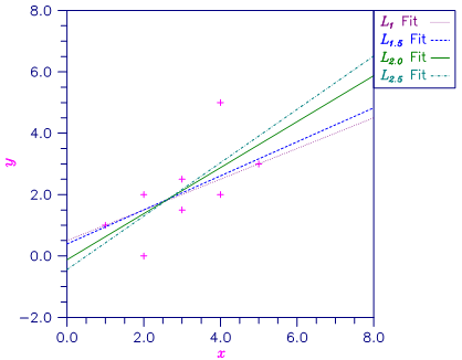
Figure 12, Various Lp Fitted Lines
Published date: 03/19/2020
Last modified date: 03/19/2020


