AONEC
Analyzes a one-way classification model with covariates.
Required Arguments
NI — Vector of length NGROUP containing the number of responses for each group. (Input)
XY — (NI(1) + NI(2) + … + NI(NGROUP)) by (NCOV + 1) matrix containing the data for each covariate and the response variable. (Input)
Data for each group must appear in contiguous rows of XY, and the responses must appear in the last column.
Data for each group must appear in contiguous rows of XY, and the responses must appear in the last column.
AOV — Vector of length 15 that contains statistics relating to the analysis of variance for the model assuming parallelism. (Output)
I | AOV(I) |
|---|---|
1 | Degrees of freedom for model (groups + covariates) |
2 | Degrees of freedom for error |
3 | Total (corrected) degrees of freedom |
4 | Sum of squares for model |
5 | Sum of squares for error |
6 | Total (corrected) sum of squares |
7 | Model mean square |
8 | Error mean square |
9 | F -statistic |
10 | p-value |
11 | R2 (in percent) |
12 | Adjusted R2 (in percent) |
13 | Estimate of the error standard deviation |
14 | Overall response mean |
15 | Coefficient of variation (in percent) |
Optional Arguments
NGROUP — Number of groups. (Input)
Default: NGROUP = size (NI,1).
Default: NGROUP = size (NI,1).
NCOV — Number of covariates. (Input)
Default: NCOV = size (XY,2) – 1.
Default: NCOV = size (XY,2) – 1.
LDXY — Leading dimension of XY exactly as specified in the dimension statement in the calling program. (Input)
Default: LDXY = size (XY,1).
Default: LDXY = size (XY,1).
ITEST — Indicator for test for parallelism (equal covariate coefficients across groups). (Input)
Default: ITEST = 0.
Default: ITEST = 0.
ITEST | Action |
|---|---|
0 | Test for parallelism is not performed. |
1 | Test for parallelism is performed. |
IPRINT — Printing option. (Input)
Default: IPRINT = 0.
Default: IPRINT = 0.
IPRINT | Action |
|---|---|
0 | No printing is performed. |
1 | Printing for model assuming parallelism is performed. |
2 | Printing for separate regression models for each group is performed as well as for the model assuming parallelism. |
COEF — NGROUP + NCOV by 4 matrix containing statistics relating to the regression coefficients for the model assuming parallelism. (Output)
Each row corresponds to a coefficient in the model. For I = 1, 2, …, NGROUP, row I is for the Y intercept for the I-th group. The remaining NCOV rows are for the covariate coefficients. The statistics in the columns are as follows:
Each row corresponds to a coefficient in the model. For I = 1, 2, …, NGROUP, row I is for the Y intercept for the I-th group. The remaining NCOV rows are for the covariate coefficients. The statistics in the columns are as follows:
Col. | Description |
|---|---|
1 | Coefficient estimate |
2 | Estimated standard error of the estimate |
3 | t-statistic |
4 | p-value |
LDCOEF — Leading dimension of COEF exactly as specified in the dimension statement in the calling program. (Input)
Default: LDCOEF = size (COEF,1).
Default: LDCOEF = size (COEF,1).
R — NGROUP + NCOV by NGROUP + NCOV upper triangular matrix containing the R matrix from the QR decomposition. (Output)
The R matrix is from the regression assuming parallelism.
The R matrix is from the regression assuming parallelism.
LDR — Leading dimension of R exactly as specified in the dimension statement in the calling program. (Input)
Default: LDR = size (R,1).
Default: LDR = size (R,1).
PTSS — Vector of length 8 containing statistics relating to the partial sums of squares for groups and for covariates in the model assuming parallelism. (Output)
I | PTSS(I) |
|---|---|
1 | Degrees of freedom for groups after covariates |
2 | Degrees of freedom for covariates after groups |
3 | Sum of squares for groups after covariates |
4 | Sum of squares for covariates after groups |
5 | F -statistic for groups |
6 | F -statistic for covariates |
7 | p-value for groups |
8 | p-value for covariates |
TESTPL — Vector of length 10 containing statistics relating to the test for parallelism. (Output if ITEST = 1)
If ITEST = 0, TESTPL is not referenced and can be a vector of length one.
If ITEST = 0, TESTPL is not referenced and can be a vector of length one.
I | TESTPL(I) |
|---|---|
1 | Extra degrees of freedom for model not assuming parallelism |
2 | Degrees of freedom for error for model not assuming parallelism |
3 | Degrees of freedom for error for model assuming parallelism |
4 | Extra sum of squares for model not assuming parallelism |
5 | Sum of squares for error for model not assuming parallelism |
6 | Sum of squares for error for model assuming parallelism |
7 | Mean square for TESTPL(1) |
8 | Mean square for TESTPL(2) |
9 | F -statistic |
10 | p-value |
XYMEAN — NGROUP + 1 by NCOV + 3 matrix containing means. (Output)
Each row for I = 1, 2, …, NGROUP corresponds to a group. Row NGROUP + 1 contains overall statistics. The statistics in the columns are as follows:
Each row for I = 1, 2, …, NGROUP corresponds to a group. Row NGROUP + 1 contains overall statistics. The statistics in the columns are as follows:
Column | Description |
|---|---|
1 | Number of nonmissing cases. |
2 thru NCOV+1 | Covariate means. |
NCOV + 2 | Response mean. |
NCOV + 3 | Adjusted mean assuming parallelism |
LDXYME — Leading dimension of XYMEAN exactly as specified in the dimension statement in the calling program. (Input)
Default: LDXYME = size (XYMEAN,1).
Default: LDXYME = size (XYMEAN,1).
COVM — NGROUP by NGROUP matrix containing the estimated variance-covariance matrix of the adjusted group means in the model assuming parallelism. (Output)
LDCOVM — Leading dimension of COVM exactly as specified in the dimension statement in the calling program. (Input)
Default: LDCOVM = size (COVM,1).
Default: LDCOVM = size (COVM,1).
COVB — NGROUP + NCOV by NGROUP + NCOV matrix containing the estimated variance-covariance matrix of the estimated coefficients in the model assuming parallelism. (Output)
If R is not needed, R and COVB can occupy the same storage locations.
If R is not needed, R and COVB can occupy the same storage locations.
LDCOVB — Leading dimension of COVB exactly as specified in the dimension statement in the calling program. (Input)
Default: LDCOVB = size (COVB,1).
Default: LDCOVB = size (COVB,1).
NRMISS — Number of rows of XY that contain any missing values. (Output)
Rows of XY containing NaN (not a number) are omitted from computations.
Rows of XY containing NaN (not a number) are omitted from computations.
FORTRAN 90 Interface
Generic: CALL AONEC (NI, XY, AOV [, …])
Specific: The specific interface names are S_AONEC and D_AONEC.
FORTRAN 77 Interface
Single: CALL AONEC (NGROUP, NI, NCOV, XY, LDXY, ITEST, IPRINT, COEF, LDCOEF, R, LDR, AOV, PTSS, TESTPL, XYMEAN, LDXYME, COVM, LDCOVM, COVB, LDCOVB, NRMISS)
Double: The double precision name is DAONEC.
Description
Routine AONEC performs analyses for models that combine the features of a one-way analysis of variance model with that of a multiple linear regression model. The basic one-way analysis of covariance model is
where the observed value of yij constitutes the j-th response in the i-th group, β0 ι denotes the y intercept for the regression function for the i-th group, β1, β2, …, βm are the regression coefficients for the covariates, and the ɛ ij’s are independently distributed normal errors with mean zero and variance σ2. This model allows the regression function for each group to have different intercepts. However, the remaining m regression coefficients are the same for each group, i.e., the regression functions are parallel. Often in practice, the regression functions are not parallel. In addition to estimates for the model assuming parallelism, AONEC computes estimates and summary statistics for the separate regressions for each group. With IPRINT = 2, the estimates and summary statistics for each group are printed. If ITEST = 1, a test for parallelism is performed.
AONEC requires (xij1, xij2, …, xijk, yij) as input into a single data matrix XY with the data for each group occupying contiguous rows of XY.
Estimates for the β0i’s and β1, β2, …, βm in the model assuming parallelism are computed and stored in COEF. Summary statistics are also computed for this model. The adjusted group means (stored in column m + 3 of XYMEAN) are given by
The estimated covariance between the i1-th and i2-th adjusted group mean is given by
where vpq is the pq-th entry in COVB and is the estimated covariance between the p-th and q-th estimated coefficients in the regression function.
The design of AONEC can be used with routines described in Chapter 2, “Regression.” For example, confidence intervals and diagnostics for the individual cases can be computed by using the output matrices R and COEF as input into regression routines for case analysis.
A discussion of formulas and interpretations for the one-way analysis of covariance problem appears in most elementary statistics texts, e.g., Snedecor and Cochran (1967, Chapter 14).
Comments
Workspace may be explicitly provided, if desired, by use of A2NEC/DA2NEC. The reference is:
CALL A2NEC (NGROUP, NI, NCOV, XY, LDXY, ITEST, IPRINT, COEF, LDCOEF, R, LDR, AOV, PTSS, TESTPL, XYMEAN, LDXYME, COVM, LDCOVM, COVB, LDCOVB, NRMISS, WK)
The additional argument is:
WK — Work vector of length 4 * (NGROUP + NCOV + 1).
Examples
Example 1
This example fits a one-way analysis of covariance model assuming parallelism using data discussed by Snedecor and Cochran (Table 14.6.1, pages 432‑436). The responses are concentrations of cholesterol (in mg/100 ml) in the blood of two groups of women: women from Iowa and women from Nebraska. Age of a woman is the single covariate. The cholesterol concentrations and ages of the women according to state are shown in the following table. (There are 11 Iowa women and 19 Nebraska women in the study. Only the first 5 women from each state are shown here.)
Iowa | Nebraska | ||
|---|---|---|---|
Age | Cholesterol | Age | Cholesterol |
46 | 181 | 18 | 137 |
52 | 228 | 44 | 173 |
39 | 182 | 33 | 177 |
65 | 249 | 78 | 241 |
54 | 259 | 51 | 225 |
There is no evidence from the data to indicate that the regression lines for cholesterol concentration as a function of age are not parallel for Iowa and Nebraska women (p-value is 0.5425). The parallel line model suggests that Nebraska women may have higher cholesterol concentrations than Iowa women. The cholesterol concentrations (adjusted for age) are 195.5 for Iowa women versus 224.2 for Nebraska women. The difference is 28.7 with an estimated standard error of
USE AONEC_INT
IMPLICIT NONE
INTEGER LDXY, NCOV, NGROUP, NOBS
PARAMETER (NCOV=1, NGROUP=2, NOBS=30, LDXY=NOBS)
!
INTEGER IPRINT, ITEST, NI(NGROUP)
REAL AOV(15), XY(LDXY,NCOV+1)
!
DATA NI/11, 19/
DATA XY/46.0, 52.0, 39.0, 65.0, 54.0, 33.0, 49.0, 76.0, 71.0, &
41.0, 58.0, 18.0, 44.0, 33.0, 78.0, 51.0, 43.0, 44.0, 58.0, &
63.0, 19.0, 42.0, 30.0, 47.0, 58.0, 70.0, 67.0, 31.0, 21.0, &
56.0, 181.0, 228.0, 182.0, 249.0, 259.0, 201.0, 121.0, &
339.0, 224.0, 112.0, 189.0, 137.0, 173.0, 177.0, 241.0, &
225.0, 223.0, 190.0, 257.0, 337.0, 189.0, 214.0, 140.0, &
196.0, 262.0, 261.0, 356.0, 159.0, 191.0, 197.0/
!
ITEST = 1
IPRINT = 2
CALL AONEC (NI, XY, AOV, ITEST=ITEST, IPRINT=IPRINT)
!
END
Output
SEPARATE REGRESSION FOR GROUP 1
Dependent R-squared Adjusted Est. Std. Dev. Coefficient of
Variable (percent) R-squared of Model Error Mean Var. (percent)
Y 47.120 41.245 48.9 207.7 23.54
* * * Analysis of Variance * * *
Sum of Mean Prob. of
Source DF Squares Square Overall F Larger F
Model 1 19177.2 19177.2 8.020 0.0197
Error 9 21521.0 2391.2
Corrected Total 10 40698.2
Inference on Coefficients
Standard Prob. of
Coef. Estimate Error t-statistic Larger |t|
1 35.81 62.47 0.573 0.5805
2 3.24 1.14 2.832 0.0197
SEPARATE REGRESSION FOR GROUP 2
Dependent R-squared Adjusted Est. Std. Dev. Coefficient of
Variable (percent) R-squared of Model Error Mean Var. (percent)
Y 56.812 54.272 39.76 217.1 18.31
* * * Analysis of Variance * * *
Sum of Mean Prob. of
Source DF Squares Square Overall F Larger F
Model 1 35351.9 35351.9 22.363 0.0002
Error 17 26873.9 1580.8
Corrected Total 18 62225.8
Inference on Coefficients
Standard Prob. of
Coef. Estimate Error t-statistic Larger |t|
1 101.3 26.13 3.876 0.0012
2 2.5 0.53 4.729 0.0002
SAME REGRESSION FOR ALL GROUPS
Dependent R-squared Adjusted Est. Std. Dev. Coefficient of
Variable (percent) R-squared of Model Error Mean Var. (percent)
Y 47.303 45.421 44.14 213.7 20.66
* * * Analysis of Variance * * *
Sum of Mean Prob. of
Source DF Squares Square Overall F Larger F
Model 1 48976.3 48976.3 25.134 0.0000
Error 28 54560.4 1948.6
Corrected Total 29 103536.7
Inference on Coefficients
Standard Prob. of
Coef. Estimate Error t-statistic Larger |t|
1 91.57 25.65 3.570 0.0013
2 2.51 0.50 5.013 0.0000
REGRESSION ASSUMING PARALLELISM
Dependent R-squared Adjusted Est. Std. Dev. Coefficient of
Variable (percent) R-squared of Model Error Mean Var. (percent)
Y 52.573 49.060 42.65 213.7 19.96
* * * Analysis of Variance * * *
Sum of Mean Prob. of
Source DF Squares Square Overall F Larger F
Model 2 54432.8 27216.4 14.965 0.0000
Error 27 49103.9 1818.7
Corrected Total 29 103536.7
Partial Sums of Squares
Sum of Prob. of
Source DF Squares F Larger F
Groups after
Covariates 1 5456.5 3.000 0.0947
Covariates after
Groups 1 53820.1 29.593 0.0000
R Matrix
1 2 3
1 3.3 0.0 176.1
2 4.4 200.3
3 86.0
Inference on Coefficients
Standard Prob. of
Coef. Estimate Error t-statistic Larger |t|
1 64.49 29.3 2.201 0.0365
2 93.14 24.8 3.756 0.0008
3 2.70 0.5 5.440 0.0000
Test for Parallelism
Sum of Mean Prob. of
Source DF Squares Square F Larger F
Extra due to
nonparallelism 1 709.0 709.0 0.381 0.5425
Error assuming
nonparallelism 26 48394.9 1861.3
Error assuming
parallelism 27 49103.9
XYMEAN
1 2 3 4
1 11 53.09 207.7 195.5
2 19 45.95 217.1 224.2
3 30 48.57 213.7 213.7
Variance-Covariance Matrix of the Adjusted Group Means
1 2
1 170.4 -2.9
2 97.4
Variance-Covariance Matrix of the Estimated Coefficients
1 2 3
1 858.6 600.0 -13.1
2 615.0 -11.3
3 0.2
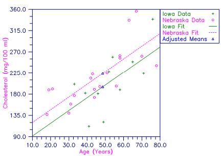
Figure 14, Plot of Cholesterol Concentrations and Fitted Parallel Lines by State
Example 2
This example fits a one-way analysis of covariance model and performs a test for parallelism using data discussed by Snedecor and Cochran (1967, Table 14.8.1, pages 438‑443). The responses are weight gains (in pounds per day) of 40 pigs for 4 groups of pigs under varying treatments. Two covariates-initial age (in days) and initial weight (in pounds)‑are used. For each treatment, there are 10 pigs. Only the first 5 pigs from each treatment are shown here.
Treatment 1 | Treatment 2 | Treatment 3 | Treatment 4 | ||||||||
|---|---|---|---|---|---|---|---|---|---|---|---|
Age | Wt. | Gain | Age | Wt. | Gain | Age | Wt. | Gain | Age | Wt. | Gain |
78 | 61 | 1.40 | 78 | 74 | 1.61 | 78 | 80 | 1.67 | 77 | 62 | 1.40 |
90 | 59 | 1.79 | 99 | 75 | 1.31 | 83 | 61 | 1.41 | 71 | 55 | 1.47 |
94 | 76 | 1.72 | 80 | 64 | 1.12 | 79 | 62 | 1.73 | 78 | 62 | 1.37 |
71 | 50 | 1.47 | 75 | 48 | 1.35 | 70 | 47 | 1.23 | 70 | 43 | 1.15 |
99 | 61 | 1.26 | 94 | 62 | 1.29 | 85 | e59 | 1.49 | 95 | 57 | 1.22 |
USE AONEC_INT
IMPLICIT NONE
INTEGER LDXY, NCOV, NGROUP, NOBS
PARAMETER (NCOV=2, NGROUP=4, NOBS=40, LDXY=NOBS)
!
INTEGER IPRINT, ITEST, NI(NGROUP)
REAL AOV(15), XY(LDXY,NCOV+1)
!
DATA NI/10, 10, 10, 10/
DATA XY/78.0, 90.0, 94.0, 71.0, 99.0, 80.0, 83.0, 75.0, 62.0, &
67.0, 78.0, 99.0, 80.0, 75.0, 94.0, 91.0, 75.0, 63.0, 62.0, &
67.0, 78.0, 83.0, 79.0, 70.0, 85.0, 83.0, 71.0, 66.0, 67.0, &
67.0, 77.0, 71.0, 78.0, 70.0, 95.0, 96.0, 71.0, 63.0, 62.0, &
67.0, 61.0, 59.0, 76.0, 50.0, 61.0, 54.0, 57.0, 45.0, 41.0, &
40.0, 74.0, 75.0, 64.0, 48.0, 62.0, 42.0, 52.0, 43.0, 50.0, &
40.0, 80.0, 61.0, 62.0, 47.0, 59.0, 42.0, 47.0, 42.0, 40.0, &
40.0, 62.0, 55.0, 62.0, 43.0, 57.0, 51.0, 41.0, 40.0, 45.0, &
39.0, 1.40, 1.79, 1.72, 1.47, 1.26, 1.28, 1.34, 1.55, 1.57, &
1.26, 1.61, 1.31, 1.12, 1.35, 1.29, 1.24, 1.29, 1.43, 1.29, &
1.26, 1.67, 1.41, 1.73, 1.23, 1.49, 1.22, 1.39, 1.39, 1.56, &
1.36, 1.40, 1.47, 1.37, 1.15, 1.22, 1.48, 1.31, 1.27, 1.22, &
1.36/
!
ITEST = 1
IPRINT = 2
CALL AONEC (NI, XY, AOV, ITEST=ITEST, IPRINT=IPRINT)
!
END
Output
SEPARATE REGRESSION FOR GROUP 1
Dependent R-squared Adjusted Est. Std. Dev. Coefficient of
Variable (percent) R-squared of Model Error Mean Var. (percent)
Y 13.271 0.000 0.2013 1.464 13.75
* * * Analysis of Variance * * *
Sum of Mean Prob. of
Source DF Squares Square Overall F Larger F
Model 2 0.0434 0.02170 0.536 0.6075
Error 7 0.2836 0.04052
Corrected Total 9 0.3270
Inference on Coefficients
Standard Prob. of
Coef. Estimate Error t-statistic Larger |t|
1 1.357 0.4639 2.925 0.0222
2 -0.006 0.0105 -0.572 0.5849
3 0.011 0.0114 0.948 0.3749
SEPARATE REGRESSION FOR GROUP 2
Dependent R-squared Adjusted Est. Std. Dev. Coefficient of
Variable (percent) R-squared of Model Error Mean Var. (percent)
Y 21.989 0.000 0.1292 1.319 9.799
* * * Analysis of Variance * * *
Sum of Mean Prob. of
Source DF Squares Square Overall F Larger F
Model 2 0.0330 0.01648 0.987 0.4193
Error 7 0.1169 0.01670
Corrected Total 9 0.1499
Inference on Coefficients
Standard Prob. of
Coef. Estimate Error t-statistic Larger |t|
1 1.401 0.2694 5.199 0.0013
2 -0.005 0.0040 -1.164 0.2825
3 0.005 0.0040 1.301 0.2343
SEPARATE REGRESSION FOR GROUP 3
Dependent R-squared Adjusted Est. Std. Dev. Coefficient of
Variable (percent) R-squared of Model Error Mean Var. (percent)
Y 49.246 34.745 0.1369 1.445 9.473
* * * Analysis of Variance * * *
Sum of Mean Prob. of
Source DF Squares Square Overall F Larger F
Model 2 0.1273 0.06364 3.396 0.0931
Error 7 0.1312 0.01874
Corrected Total 9 0.2584
Inference on Coefficients
Standard Prob. of
Coef. Estimate Error t-statistic Larger |t|
1 1.452 0.4709 3.082 0.0178
2 -0.008 0.0075 -1.017 0.3429
3 0.011 0.0043 2.544 0.0384
SEPARATE REGRESSION FOR GROUP 4
Dependent R-squared Adjusted Est. Std. Dev. Coefficient of
Variable (percent) R-squared of Model Error Mean Var. (percent)
Y 17.076 0.000 0.1141 1.325 8.609
* * * Analysis of Variance * * *
Sum of Mean Prob. of
Source DF Squares Square Overall F Larger F
Model 2 0.0188 0.00938 0.721 0.5193
Error 7 0.0911 0.01301
Corrected Total 9 0.1098
Inference on Coefficients
Standard Prob. of
Coef. Estimate Error t-statistic Larger |t|
1 1.044 0.2574 4.055 0.0048
2 0.001 0.0038 0.251 0.8094
3 0.004 0.0051 0.833 0.4324
SAME REGRESSION FOR ALL GROUPS
Dependent R-squared Adjusted Est. Std. Dev. Coefficient of
Variable (percent) R-squared of Model Error Mean Var. (percent)
Y 17.724 13.277 0.1508 1.388 10.86
* * * Analysis of Variance * * *
Sum of Mean Prob. of
Source DF Squares Square Overall F Larger F
Model 2 0.181 0.09064 3.985 0.0271
Error 37 0.842 0.02274
Corrected Total 39 1.023
Inference on Coefficients
Standard Prob. of
Coef. Estimate Error t-statistic Larger |t|
1 1.251 0.1708 7.327 0.0000
2 -0.003 0.0028 -1.178 0.2464
3 0.007 0.0027 2.743 0.0093
REGRESSION ASSUMING PARALLELISM
Dependent R-squared Adjusted Est. Std. Dev. Coefficient of
Variable (percent) R-squared of Model Error Mean Var. (percent)
Y 34.467 24.829 0.1404 1.388 10.11
* * * Analysis of Variance * * *
Sum of Mean Prob. of
Source DF Squares Square Overall F Larger F
Model 5 0.353 0.07050 3.576 0.0105
Error 34 0.670 0.01971
Corrected Total 39 1.023
Partial Sums of Squares
Sum of Prob. of
Source DF Squares F Larger F
Groups after
Covariates 3 0.1712 2.895 0.0493
Covariates after
Groups 2 0.1750 4.438 0.0194
R Matrix
1 2 3 4 5 6
1 3.2 0.0 0.0 0.0 252.7 172.0
2 3.2 0.0 0.0 247.9 173.9
3 3.2 0.0 236.9 164.4
4 3.2 237.2 156.5
5 67.4 42.7
6 55.3
Inference on Coefficients
Standard Prob. of
Coef. Estimate Error t-statistic Larger |t|
1 1.337 0.1724 7.751 0.0000
2 1.182 0.1697 6.965 0.0000
3 1.318 0.1626 8.109 0.0000
4 1.217 0.1624 7.493 0.0000
5 -0.003 0.0026 -1.314 0.1978
6 0.007 0.0025 2.919 0.0062
Test for Parallelism
Sum of Mean Prob. of
Source DF Squares Square F Larger F
Extra due to
nonparallelism 6 0.0474 0.00790 0.355 0.9007
Error assuming
nonparallelism 28 0.6228 0.02224
Error assuming
parallelism 34 0.6703
XYMEAN
1 2 3 4 5
1 10 79.90 54.40 1.464 1.461
2 10 78.40 55.00 1.319 1.307
3 10 74.90 52.00 1.445 1.443
4 10 75.00 49.50 1.325 1.342
5 40 77.05 52.72 1.388 1.388
Variance-Covariance Matrix of the Adjusted Group Means
1 2 3 4
1 0.002007 0.000016 -0.000027 -0.000024
2 0.001992 -0.000007 -0.000030
3 0.001994 0.000011
4 0.002014
Variance-Covariance Matrix of the Estimated Coefficients
1 2 3 4 5 6
1 0.02974 0.02729 0.02605 0.02602 -0.00033 -0.00002
2 0.02880 0.02561 0.02556 -0.00032 -0.00003
3 0.02642 0.02441 -0.00031 -0.00003
4 0.02638 -0.00032 -0.00001
5 0.00001 0.00000
6 0.00001
Published date: 03/19/2020
Last modified date: 03/19/2020


