DESPL

Performs nonparametric probability density function estimation by the penalized likelihood method.
Required Arguments
X — Vector of length NOBS containing the random sample of responses. (Input)
NODE — Number of mesh nodes for the discrete probability density estimate. (Input)
NODE must be an odd integer greater than 4.
NODE must be an odd integer greater than 4.
BNDS — Vector of length 2 containing the upper and lower endpoints for the interval of support of the density. (Input)
The node values are taken as BNDS(1), BNDS(1) + h, …, BNDS(2), where h = (BNDS(2) ‑ BNDS(1))/(NODE ‑ 1). All observations in vector X should be in the support interval.
The node values are taken as BNDS(1), BNDS(1) + h, …, BNDS(2), where h = (BNDS(2) ‑ BNDS(1))/(NODE ‑ 1). All observations in vector X should be in the support interval.
DENS — Vector of length NODE containing the estimated values of the discrete pdf at the NODE equally spaced mesh nodes. (Input/Output, if INIT ≠ 0; Output, otherwise)
If INIT is not zero, then DENS(1) through DENS(NODE) contain the (positive) initial estimates on input. The sum of these estimates times the window width h (see BNDS) must equal 1.0, i.e., the integral of the density must be 1.
If INIT is not zero, then DENS(1) through DENS(NODE) contain the (positive) initial estimates on input. The sum of these estimates times the window width h (see BNDS) must equal 1.0, i.e., the integral of the density must be 1.
STAT — Vector of length 4 containing output statistics. (Output)
STAT(1) and STAT(2) contain the log‑likelihood and the log‑penalty terms, respectively. STAT(3) and STAT(4) contain the estimated mean and variance for the estimated density.
STAT(1) and STAT(2) contain the log‑likelihood and the log‑penalty terms, respectively. STAT(3) and STAT(4) contain the estimated mean and variance for the estimated density.
Optional Arguments
NOBS — Number of observations. (Input)
Default: NOBS = size (X,1).
Default: NOBS = size (X,1).
INIT — Initialization option. (Input)
INIT = 0 means that a bootstrap procedure is used to obtain initial estimates for the density. Otherwise, user‑supplied initial estimates are contained in DENS on entry into DESPL.
Default: INIT = 0.
INIT = 0 means that a bootstrap procedure is used to obtain initial estimates for the density. Otherwise, user‑supplied initial estimates are contained in DENS on entry into DESPL.
Default: INIT = 0.
ALPHA — Penalty‑weighting factor that controls the smoothness of the estimate. (Input)
For standard normal data, ALPHA = 10.0 works well. Other values that might be tried are 1.0 and 100.0. ALPHA must be greater than 0.0.
Default: ALPHA = 10.0.
For standard normal data, ALPHA = 10.0 works well. Other values that might be tried are 1.0 and 100.0. ALPHA must be greater than 0.0.
Default: ALPHA = 10.0.
MAXIT — Maximum number of iterations allowed in the iterative procedure. (Input)
MAXIT = 30 is typical.
Default: MAXIT = 30.
MAXIT = 30 is typical.
Default: MAXIT = 30.
EPS — Convergence criterion. (Input)
When the Euclidean norm of the changes to DENS is less than EPS, convergence is assumed. EPS = 0.0001 is typical.
Default: EPS = 0.0001.
When the Euclidean norm of the changes to DENS is less than EPS, convergence is assumed. EPS = 0.0001 is typical.
Default: EPS = 0.0001.
NMISS — Number of missing values in X. (Output)
FORTRAN 90 Interface
Generic: CALL DESPL (X, NODE, BNDS, DENS, STAT [, …])
Specific: The specific interface names are S_DESPL and D_DESPL.
FORTRAN 77 Interface
Single: CALL DESPL (NOBS, X, NODE, BNDS, INIT, ALPHA, MAXIT, EPS, DENS, STAT, NMISS)
Double: The double precision name is DDESPL.
Description
Routine DESPL computes piecewise linear estimates of a one‑dimensional density function for a given random sample of observations. These estimates are discussed in detail in Scott et al. (1980), and in Tapia and Thompson (1978, Chapter 5). The estimator of the density function is piecewise linear over the finite interval (BNDS(1) to BNDS(2)), is nonnegative, and integrates to one. A penalty method is used to ensure “smooth” behavior of the estimator. The criterion function to be maximized is a discrete approximation to
where n = NOBS and f(t) is a density function. Let m = NODE. The discrete approximation is as follows: The density f is estimated at each of the equally spaced grid points tj, for j = 1, …, m, with restriction f(t1) = f(tm) = 0.0; the density at each data point xi is then estimated using linear interpolation. The integral of the second derivative of the square of f is approximated using the piecewise linear function defined by the estimates of f at the grid points tj.
Because ln Φ is actually maximized, the criterion can be separated into a likelihood term (returned in STAT(1)) and a penalty term (returned in STAT(2)).
The parameter α (= ALPHA) determines the amount of “smoothness” in the estimate. The larger the value of α, the smoother the resulting estimator for f. In practice, the user should pick α as small as possible such that there is not excessive bumpiness in the estimator. One way of doing this is to try several values of α that differ by factors of 10. The resulting estimators can then be graphically displayed and examined for bumpiness. α could then be chosen from the displayed density estimates. IMSL routines can be used to produce line printer plots (PLOTP) of the estimated density. For a random sample from the standard normal distribution, α = 10.0 works well. Note that α changes with scale. If x is multiplied by a factor β, α should be multiplied by a factor β5.
The second choice to be made in using DESPL is the mesh for the estimator. The mesh interval (BNDS(1), BNDS(2)) should be picked as narrow as possible since a narrow mesh will speed algorithm convergence. Note, however, that points outside the interval (BNDS(1), BNDS(2)) are not included in the likelihood. Because of this fact, DESPL actually estimates a density that is conditional on the mesh interval (BNDS(1), BNDS(2)). The number of mesh nodes, NODE, should be as small as possible, but large enough to exhibit the “fine” structure of the density. One possible method for determining NODE is to use NODE = 21 initially. With NODE = 21, find an acceptable value for α. When an acceptable value for α has been found, increase or decrease NODE as required.
STAT(3) and STAT(4) contain “exact” estimates of the mean and variance when the estimated piecewise linear density is used in the required integrals. Routine DESPT may be used to find interpolated estimates for the density at any point x given the NODE estimates of the density returned in DENS.
Comments
1. Workspace may be explicitly provided, if desired, by use of D2SPL/DD2SPL. The reference is:
CALL D2SPL (NOBS, X, NODE, BNDS, INIT, ALPHA, MAXIT, EPS, DENS, STAT, NMISS, HESS, LDHESS, ILOHI, DENEST, B, IPVT, WK2, XWK)
The additional arguments are as follows:
HESS — Work vector of length 7 * (NODE – 2).
LDHESS — Leading dimension of HESS exactly as specified in the dimension statement in the calling program. (Input)
The leading dimension must be set to 7.
The leading dimension must be set to 7.
ILOHI — Integer work vector of length 2 * NODE.
DENEST — Work vector of length 3 * NODE.
B — Work vector of length NODE.
IPVT — Integer work vector of length NODE ‑ 2.
WK2 — Work vector of length NODE – 2.
XWK — Work vector of length NOBS. If X is sorted with all missing (NaN, not a number) values at the end, then XWK is not needed. If X is not needed, X and XWK can share the same storage location.
2. Informational error
Type | Code | Description |
|---|---|---|
3 | 1 | The maximum number of iterations is exceeded. |
3 Routine DESPT may be used after the estimates DENS have been obtained in order to obtain an interpolated estimate of the density at new points. Use AMESH = BNDS in calling DESPT.
Example
An estimate for a density function of unknown form using a random sample of size 10 and 13 mesh points with α = 10 is estimated as follows:
USE DESPL_INT
USE UMACH_INT
IMPLICIT NONE
INTEGER NOBS, NODE
PARAMETER (NOBS=10, NODE=13)
!
INTEGER NOUT
REAL BNDS(2), DENS(NODE), STAT(4), X(NOBS)
!
DATA BNDS/-3., 3./
DATA X/-.9471, -.7065, -.2933, -.1169, .2217, .4425, .4919, &
.5752, 1.1439, 1.3589/
!
CALL DESPL (X, NODE, BNDS, DENS, STAT)
!
CALL UMACH (2, NOUT)
WRITE (NOUT,'('' DENS = '',9F7.4, /, 9X, 4F7.4)') DENS
WRITE (NOUT,'('' Log-likelihood term = '', F7.3, /, &
'' Log-penalty term = '', F7.3, /, &
'' Mean = '', F7.3, /, &
'' Variance = '', F7.3)') STAT
END
Output
DENS = 0.0000 0.0014 0.0356 0.1111 0.2132 0.3040 0.3575 0.3565 0.2947
0.1986 0.0986 0.0288 0.0000
Log-likelihood term = -11.968
Log-penalty term = -1.303
Mean = 0.217
Variance = 1.042
The following figure shows the affect of various choices of α. For larger α, the density estimate is smoother.
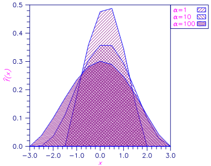
Figure 20, Density Estimates Using α = 1, 10, 100


