RONE
Analyzes a simple linear regression model.
Required Arguments
X — NOBS by NCOL matrix containing the data. (Input)
IRSP — Column number IRSP of X contains the data for the response (dependent) variable. (Input)
IND — Column number IND of X contains the data for the independent (explanatory) variable. (Input)
AOV — Vector of length 15 containing statistics relating to the analysis of variance. (Output)
I | AOV(I) |
1 | Degrees of freedom for regression |
2 | Degrees of freedom for error |
3 | Total degrees of freedom |
4 | Sum of squares for regression |
5 | Sum of squares for error |
6 | Total sum of squares |
7 | Regression mean square |
8 | Error mean square |
9 | F-statistic |
10 | p‑value |
11 | R2 (in percent) |
12 | Adjusted R2 (in percent) |
13 | Estimated standard deviation of the model error |
14 | Mean of the response (dependent) variable |
15 | Coefficient of variation (in percent) |
If INTCEP = 1, the regression and total are corrected for the mean. If INTCEP = 0, the regression and total are not corrected for the mean, and AOV(14) and AOV(15) are set to NaN (not a number).
COEF — INTCEP + 1 by 5 matrix containing statistics relating the regression coefficients. (Output)
If INTCEP = 1, the first row corresponds to the intercept. Row INTCEP + 1 corresponds to the coefficient for the slope. The statistics in the columns are
If INTCEP = 1, the first row corresponds to the intercept. Row INTCEP + 1 corresponds to the coefficient for the slope. The statistics in the columns are
Col. | Description |
1 | Coefficient estimate |
2 | Estimated standard error of the coefficient estimate |
3 | t-statistic for the test that the coefficient is zero |
4 | p‑value for the two-sided t test |
5 | Variance inflation factor |
COVB — INTCEP + 1 by INTCEP + 1 matrix that is the estimated variance-covariance matrix of the estimated regression coefficients. (Output)
TESTLF — Vector of length 10 containing statistics relating to the test for lack of fit of the model. (Output)
Elem | Description |
1 | Degrees of freedom for lack of fit |
2 | Degrees of freedom for pure error |
3 | Degrees of freedom for error (TESTLF(1) + TESTLF(2)) |
4 | Sum of squares for lack of fit |
5 | Sum of squares for pure error |
6 | Sum of squares for error |
7 | Mean square for lack of fit |
8 | Mean square for pure error |
9 | F statistic |
10 | p‑value |
If there are no replicates in the data set, a test for lack of fit cannot be performed. In this case, elements 7, 8, 9, and 10 of TESTLF are set to NaN (not a number).
CASE — NOBS by 12 matrix containing case statistics. (Output)
Columns 1 through 12 contain the following:
Columns 1 through 12 contain the following:
Col. | Description |
1 | Observed response |
2 | Predicted response |
3 | Residual |
4 | Leverage |
5 | Standardized residual |
6 | Jackknife residual |
7 | Cook’s distance |
8 | DFFITS |
9, 10 | Confidence interval on the mean |
11, 12 | Prediction interval |
Optional Arguments
NOBS — Number of observations. (Input)
Default: NOBS = size (X,1).
Default: NOBS = size (X,1).
NCOL — Number of columns in X. (Input)
Default: NCOL = size (X,2).
Default: NCOL = size (X,2).
LDX — Leading dimension of X exactly as specified in the dimension statement in the calling program. (Input)
Default: LDX = size (X,1).
Default: LDX = size (X,1).
INTCEP — Intercept option. (Input)
Default: INTCEP = 1.
Default: INTCEP = 1.
INTCEP | Action |
|---|---|
0 | An intercept is not in the model. |
1 | An intercept is in the model. |
IFRQ — Frequency option. (Input)
IFRQ = 0 means that all frequencies are 1.0. For positive IFRQ, column number IFRQ of X contains the frequencies. If X(I, IFRQ) = 0.0, none of the remaining elements of row I of X are referenced, and updating of statistics is skipped for row I.
Default: IFRQ = 0.
IFRQ = 0 means that all frequencies are 1.0. For positive IFRQ, column number IFRQ of X contains the frequencies. If X(I, IFRQ) = 0.0, none of the remaining elements of row I of X are referenced, and updating of statistics is skipped for row I.
Default: IFRQ = 0.
IWT — Weighting option. (Input)
IWT = 0 means that all weights are 1.0. For positive IWT, column number IWT of X contains the weights.
Default: IWT = 0.
IWT = 0 means that all weights are 1.0. For positive IWT, column number IWT of X contains the weights.
Default: IWT = 0.
IPRED — Prediction interval option. (Input)
IPRED = 0 means that prediction intervals are computed for a single future response. For positive IPRED, a prediction interval is computed on the average of future responses, and column number IPRED of X contains the number of future responses in each average.
Default: IPRED =0.
IPRED = 0 means that prediction intervals are computed for a single future response. For positive IPRED, a prediction interval is computed on the average of future responses, and column number IPRED of X contains the number of future responses in each average.
Default: IPRED =0.
CONPCM — Confidence level for two-sided interval estimates on the mean, in percent. (Input)
CONPCM percent confidence intervals are computed, hence, CONPCM must be greater than or equal to 0.0 and less than 100.0. CONPCM often will be 90.0, 95.0, or 99.0. For one-sided intervals with confidence level ONECL, where ONECL is greater than or equal to 50.0 and less than 100.0, set CONPCM = 100.0 ‑ 2.0 * (100.0 ‑ ONECL).
Default: CONPCM = 95.0.
CONPCP — Confidence level for two-sided prediction intervals, in percent. (Input)
CONPCP percent prediction intervals are computed, hence, CONPCP must be greater than or equal to 0.0 and less than 100.0. CONPCP often will be 90.0, 95.0, or 99.0. For one-sided intervals with confidence level ONECL, where ONECL is greater than or equal to 50.0 and less than 100.0, set CONPCP = 100.0 ‑ 2.0 * (100.0 ‑ ONECL).
Default: CONPCP = 95.0.
IPRINT — Printing option. (Input)
Default: IPRINT = 0.
Default: IPRINT = 0.
IPRINT | Action |
0 | No printing is performed. |
1 | AOV, COEF, TESTLF, and unusual rows of CASE are printed. |
2 | AOV, COEF, TESTLF, and unusual rows of CASE are printed. A plot of the data with the regression line is printed. |
3 | All printing is performed. A plot of the data with the regression line, a plot of the standardized residuals versus the independent variable, and a half-normal probability plot of the standardized residuals are printed. |
LDCOEF — Leading dimension of COEF exactly as specified in the dimension statement in the calling program. (Input)
Default: LDCOEF = size (COEF,1).
Default: LDCOEF = size (COEF,1).
LDCOVB — Leading dimension of COVB exactly as specified in the dimension statement in the calling program. (Input)
Default: LDCOVB = size (COVB,1).
Default: LDCOVB = size (COVB,1).
LDCASE — Leading dimension of CASE exactly as specified in the dimension statement in the calling program. (Input)
Default: LDCASE = size (CASE,1).
Default: LDCASE = size (CASE,1).
NRMISS — Number of rows of data encountered containing missing values for the independent, dependent, weight, or frequency variables. (Output)
NaN (not a number) is used as the missing value code. Any row of X containing NaN as a value of the independent, dependent, weight, or frequency variables is omitted from the computations for fitting the model.
NaN (not a number) is used as the missing value code. Any row of X containing NaN as a value of the independent, dependent, weight, or frequency variables is omitted from the computations for fitting the model.
FORTRAN 90 Interface
Generic: CALL RONE (X, IRSP, IND, AOV, COEF, COVB, TESTLF, CASE [, …])
Specific: The specific interface names are S_RONE and D_RONE.
FORTRAN 77 Interface
Single: CALL RONE (NOBS, NCOL, X, LDX, INTCEP, IRSP, IND, IFRQ, IWT, IPRED, CONPCM, CONPCP, IPRINT, AOV, COEF, LDCOEF, COVB, LDCOVB, TESTLF, CASE, LDCASE, NRMISS)
Double: The double precision name is DRONE.
Description
Routine RONE performs an analysis for the simple linear regression model. In addition to the fit, summary statistics (analysis of variance, t tests, lack-of-fit test), and confidence intervals and diagnostics for individual cases are computed. With the printing option, diagnostic plots can also be produced. Draper and Smith (1981, chapter 1) give formulas for many of the statistics computed by RONE. For definitions of the case diagnostics (stored in CASE), see the “Usage Notes” of this chapter.
Comments
1. Workspace may be explicitly provided, if desired, by use of R2NE/DR2NE. The reference is:
CALL R2NE (NOBS, NCOL, X, LDX, INTCEP, IRSP, IND, IFRQ, IWT, IPRED, CONPCM, CONPCP, IPRINT, AOV, COEF, LDCOEF, COVB, LDCOVB, TESTLF, CASE, LDCASE, NRMISS, IWK, WK)
The additional arguments are as follows:
IWK — Work vector of length NOBS.
WK — Work vector of length 3 * NOBS.
2. Informational errors
Type | Code | Description |
|---|---|---|
3 | 5 | CONPCM is less than 50.0. Confidence percentages commonly used are 90.0, 95.0, and 99.0. |
3 | 6 | CONPCP is less than 50.0. Confidence percentages commonly used are 90.0, 95.0, and 99.0. |
4 | 1 | Negative weight encountered. |
4 | 2 | Negative frequency encountered. |
4 | 7 | Each row of X contains NaN. |
Examples
Example 1
This example fits a line to a set of data discussed by Draper and Smith (1981, pages 9‑33). The response y is the amount of steam used per month (in pounds), and the independent variable x is the average atmospheric temperature (in degrees Fahrenheit). The IPRINT = 1 option is selected. Hence, plots are not produced and only unusual cases are printed. Note in the case analysis, with the default page width, the observation number and the associated 12 statistics require two lines of output. (Routine PGOPT, Chapter 19, "Utilities", can be invoked to increase the page width to put all 12 statistics on the same line.) Also note that observation 11 is labeled with a “Y” to indicate an unusual y (response). The residual for this case is about 2 standard deviations from zero.
USE RONE_INT
IMPLICIT NONE
INTEGER INTCEP, LDCASE, LDCOEF, LDCOVB, LDX, NCOEF, NCOL, NOBS
INTEGER J
PARAMETER (NOBS=25, LDX=25, LDCASE=25, INTCEP=1, NCOEF=INTCEP+1, &
LDCOEF=NCOEF, LDCOVB=NCOEF, NCOL=2)
!
INTEGER IND, IPRINT, IRSP, NRMISS
REAL AOV(15), CASE(LDCASE,12), COEF(LDCOEF,5), CONPCP, &
COVB(LDCOVB,NCOEF), TESTLF(10), X(LDX,NCOL)
!
DATA (X(1,J),J=1,2) /35.3, 10.98/
DATA (X(2,J),J=1,2) /29.7, 11.13/
DATA (X(3,J),J=1,2) /30.8, 12.51/
DATA (X(4,J),J=1,2) /58.8, 8.40/
DATA (X(5,J),J=1,2) /61.4, 9.27/
DATA (X(6,J),J=1,2) /71.3, 8.73/
DATA (X(7,J),J=1,2) /74.4, 6.36/
DATA (X(8,J),J=1,2) /76.7, 8.50/
DATA (X(9,J),J=1,2) /70.7, 7.82/
DATA (X(10,J),J=1,2) /57.5, 9.14/
DATA (X(11,J),J=1,2) /46.4, 8.24/
DATA (X(12,J),J=1,2) /28.9, 12.19/
DATA (X(13,J),J=1,2) /28.1, 11.88/
DATA (X(14,J),J=1,2) /39.1, 9.57/
DATA (X(15,J),J=1,2) /46.8, 10.94/
DATA (X(16,J),J=1,2) /48.5, 9.58/
DATA (X(17,J),J=1,2) /59.3, 10.09/
DATA (X(18,J),J=1,2) /70.0, 8.11/
DATA (X(19,J),J=1,2) /70.0, 6.83/
DATA (X(20,J),J=1,2) /74.5, 8.88/
DATA (X(21,J),J=1,2) /72.1, 7.68/
DATA (X(22,J),J=1,2) /58.1, 8.47/
DATA (X(23,J),J=1,2) /44.6, 8.86/
DATA (X(24,J),J=1,2) /33.4, 10.36/
DATA (X(25,J),J=1,2) /28.6, 11.08/
!
IRSP = 2
IND = 1
CONPCP = 99.0
IPRINT = 1
CALL RONE (X, IRSP, IND, AOV, COEF, COVB, TESTLF, CASE, &
CONPCP=CONPCP, IPRINT=IPRINT, NRMISS=NRMISS)
!
END
Output
R-squared Adjusted Est. Std. Dev. Coefficient of
(percent) R-squared of Model Error Mean Var. (percent)
71.444 70.202 0.8901 9.424 9.445
* * * Analysis of Variance * * *
Sum of Mean Prob. of
Source DF Squares Square Overall F Larger F
Regression 1 45.59 45.59 57.543 0.0000
Residual 23 18.22 0.79
Corrected Total 24 63.82
* * * Inference on Coefficients * * *
Standard Prob. of Variance
Coef. Estimate Error t-statistic Larger |t| Inflation
1 13.62 0.5815 23.43 0.0000 10.67
2 -0.08 0.0105 -7.59 0.0000 1.00
* * * Test for Lack of Fit * * *
Sum of Mean Prob. of
Source DF Squares Square Overall F Larger F
Lack of fit 22 17.40 0.7911 0.966 0.6801
Pure error 1 0.82 0.8192
Residual 23 18.22
* * * Case Analysis * * *
Obs. Observed Predicted Residual Leverage Std. Res. Jack Res.
Cook’s D DFFITS 95.0% CI 95.0% CI 99.0% PI 99.0% PI
Y 11 8.2400 9.9189 -1.6789 0.0454 -1.9305 -2.0625
0.0886 -0.4497 9.5267 10.3112 7.3640 12.4739
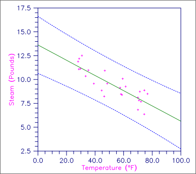
Figure 2, Plot of Line and 99% One-at-a-Time Prediction Intervals
Example 2
This example fits a line to a data set discussed by Draper and Smith (1981, pages 38‑40). The data set contains several repeated x values in order to assess lack of fit of the straight line. The IPRINT = 1 option is selected. Hence, plots are not produced and only unusual cases are printed. Note in the case analysis that observations 1 and 2 are labeled with an “X” to indicate an unusual x value. Each have leverage 0.1944 that exceeds the average leverage of p/n = 2/24 by a factor of 2.
USE RONE_INT
IMPLICIT NONE
INTEGER LDCASE, LDCOEF, LDCOVB, LDX, NCOEF, NCOL, NOBS,J
INTEGER INTCEP, NRMISS
PARAMETER (INTCEP=1, NCOL=2, NOBS=24, LDCASE=NOBS, LDX=NOBS, &
NCOEF=INTCEP+1, LDCOEF=NCOEF, LDCOVB=NCOEF)
!
INTEGER IFRQ, IND, IPRED, IPRINT, IRSP
REAL AOV(15), CASE(LDCASE,12),COEF(LDCOEF,5), &
COVB(LDCOVB,NCOEF), TESTLF(10), X(LDX,NCOL)
!
DATA (X(1,J),J=1,2) /2.3, 1.3/
DATA (X(2,J),J=1,2) /1.8, 1.3/
DATA (X(3,J),J=1,2) /2.8, 2.0/
DATA (X(4,J),J=1,2) /1.5, 2.0/
DATA (X(5,J),J=1,2) /2.2, 2.7/
DATA (X(6,J),J=1,2) /3.8, 3.3/
DATA (X(7,J),J=1,2) /1.8, 3.3/
DATA (X(8,J),J=1,2) /3.7, 3.7/
DATA (X(9,J),J=1,2) /1.7, 3.7/
DATA (X(10,J),J=1,2) /2.8, 4.0/
DATA (X(11,J),J=1,2) /2.8, 4.0/
DATA (X(12,J),J=1,2) /2.2, 4.0/
DATA (X(13,J),J=1,2) /5.4, 4.7/
DATA (X(14,J),J=1,2) /3.2, 4.7/
DATA (X(15,J),J=1,2) /1.9, 4.7/
DATA (X(16,J),J=1,2) /1.8, 5.0/
DATA (X(17,J),J=1,2) /3.5, 5.3/
DATA (X(18,J),J=1,2) /2.8, 5.3/
DATA (X(19,J),J=1,2) /2.1, 5.3/
DATA (X(20,J),J=1,2) /3.4, 5.7/
DATA (X(21,J),J=1,2) /3.2, 6.0/
DATA (X(22,J),J=1,2) /3.0, 6.0/
DATA (X(23,J),J=1,2) /3.0, 6.3/
DATA (X(24,J),J=1,2) /5.9, 6.7/
!
IRSP = 1
IND = 2
IPRINT = 1
CALL RONE (X, IRSP, IND, AOV, COEF, COVB, TESTLF, CASE, &
IPRINT=IPRINT, NRMISS=NRMISS)
END
Output
R-squared Adjusted Est. Std. Dev. Coefficient of
(percent) R-squared of Model Error Mean Var. (percent)
22.983 19.483 0.9815 2.858 34.34
* * * Analysis of Variance * * *
Sum of Mean Prob. of
Source DF Squares Square Overall F Larger F
Regression 1 6.32 6.325 6.565 0.0178
Residual 22 21.19 0.963
Corrected Total 23 27.52
* * * Inference on Coefficients * * *
Standard Prob. of Variance
Coef. Estimate Error t-statistic Larger |t| Inflation
1 1.436 0.5900 2.435 0.0235 8.672
2 0.338 0.1319 2.562 0.0178 1.000
* * * Test for Lack of Fit * * *
Sum of Mean Prob. of
Source DF Squares Square Overall F Larger F
Lack of fit 11 8.72 0.793 0.700 0.7183
Pure error 11 12.47 1.134
Residual 22 21.19
* * * Case Analysis * * *
Obs. Observed Predicted Residual Leverage Std. Res. Jack Res.
Cook’s D DFFITS 95.0% CI 95.0% CI 95.0% PI 95.0% PI
X 1 2.3000 1.8756 0.4244 0.1944 0.4817 0.4731
0.0280 0.2324 0.9783 2.7730 -0.3489 4.1002
X 2 1.8000 1.8756 -0.0756 0.1944 -0.0859 -0.0839
0.0009 -0.0412 0.9783 2.7730 -0.3489 4.1002
Y 13 5.4000 3.0245 2.3755 0.0460 2.4780 2.8515
0.1481 0.6264 2.5877 3.4612 0.9426 5.1063
Y 24 5.9000 3.7002 2.1998 0.1537 2.4363 2.7855
0.5391 1.1873 2.9021 4.4983 1.5138 5.8866

Figure 3, Plot of Leverages hi and the Average (p/n = 2/24)


