RCOMP
Generates an orthogonal central composite design.
Required Arguments
XMIN — Vector of length NVAR with the minimum values. (Input)
XMIN(i) is the minimum for the i-th variable.
XMIN(i) is the minimum for the i-th variable.
XMAX — Vector of length NVAR with the maximum values. (Input)
XMAX(i) is the maximum for the i-th variable.
XMAX(i) is the maximum for the i-th variable.
NCENTR — Number of center points. (Input)
NCENTR must be greater than 0.
NCENTR must be greater than 0.
X — NPTS by NVAR matrix containing the orthogonal central composite design. (Output)
Design settings for variable I are contained in column I of X. (I = 1, 2, …, NVAR)
Design settings for variable I are contained in column I of X. (I = 1, 2, …, NVAR)
Optional Arguments
NVAR — Number of explanatory variables. (Input)
NVAR must be greater than or equal to 2 and less than or equal to 12.
Default: NVAR = size (XMIN,1).
NVAR must be greater than or equal to 2 and less than or equal to 12.
Default: NVAR = size (XMIN,1).
IFREP — Option for the fractional replicate of the 2NVAR design selected. (Input)
IFREP is referenced only if NVAR is greater than or equal to 5. In the following table, the design points in the fractional replicate part of the design are defined using modulo 2 arithmetic. Each variable is coded 0 or 1 to represent the low and high values of the variable.
Default: IFREP = 0.
IFREP is referenced only if NVAR is greater than or equal to 5. In the following table, the design points in the fractional replicate part of the design are defined using modulo 2 arithmetic. Each variable is coded 0 or 1 to represent the low and high values of the variable.
Default: IFREP = 0.
NVAR | Defining Equations |
|---|---|
5 | |
6 | |
7 | |
8 | |
9 | |
10 | |
11 | |
12 |
NPTS — Number of design points. (Output)
NVAR | NPTS |
2 thru 4 | 2NVAR + 2 * NVAR + NCENTR |
5 thru 7 | 2NVAR−1 + 2 * NVAR + NCENTR |
8 or 9 | 2NVAR−2 + 2 * NVAR + NCENTR |
10 | 2NVAR−3 + 2 * NVAR + NCENTR |
11 or 12 | 2NVAR−4 + 2 * NVAR + NCENTR |
LDX — Leading dimension of X exactly as specified in the dimension statement in the calling program. (Input)
Default: LDX = size (X,1).
Default: LDX = size (X,1).
FORTRAN 90 Interface
Generic: CALL RCOMP (XMIN, XMAX, NCENTR, X [, …])
Specific: The specific interface names are S_RCOMP and D_RCOMP.
FORTRAN 77 Interface
Single: CALL RCOMP (NVAR, XMIN, XMAX, NCENTR, IFREP, NPTS, X, LDX)
Double: The double precision name is DRCOMP.
Description
Routine RCOMP generates an orthogonal central composite design from the minimum and maximum value for each of n (input in NVAR) variables, where 2 ≤ n ≤ 12. An orthogonal central composite design is a 2−k replicate of a 2n factorial design, i.e., a 2n−k fractional factorial, augmented by 2n axial points and m (input in NCENTR) center points. The values of n and k used by RCOMP are given by the following table:
N | k |
|---|---|
2, 3, 4 | 0 |
5, 6, 7 | 1 |
8, 9 | 2 |
10 | 3 |
11, 12 | 4 |
The fractional factorial part of all designs generated by RCOMP are of resolution V or greater. This means the fractions allow the overall mean, all the main effects, and all the two-factor interactions to be estimated. For a further discussion, see John (1971, pages 148‑157).
Experimental designs for fitting a second-order response surface must contain at least three levels of each variable in order for the regression coefficients to be estimated. Orthogonal central composite designs provide a useful alternative to the 3n factorial design, which can require an excessive number of design points. On a per observation basis, the orthogonal central composite design is no worse than the 3n factorial design with regard to efficiency for estimating the regression coefficients of the square and crossproduct variables (see Meyers 1971, pages 134‑136). The design assumes three factor and higher-way interactions are negligible.
Meyers (1971, chapter 7) and John (1971, pages 204‑206) discuss the generation of the design. The number of design points (stored in NPTS) is 2n–k + 2n + m. Each variable in the design appears at five different levels. For a second-order response surface model with the x variables coded {‑α, ‑1, 0, 1, α } and with pure quadratic terms corrected for the mean
the design produces a diagonal XTX matrix. Let
and let the minimum and maximum value of the j-th variable be denoted by x1j and x2j, respectively. The following table gives the formulas for the coded and decoded variable settings:
Coded Setting for Variable j | Decoded Setting for Variable j |
|---|---|
‑α | x1j |
‑1 | |
0 | |
1 | |
α | x2j |
Example
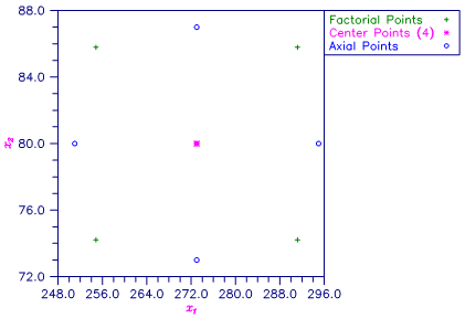
This example uses two variables and their respective minimum and maximum values to generate an orthogonal central composite design with four center points.
USE RCOMP_INT
USE UMACH_INT
USE WRRRN_INT
IMPLICIT NONE
INTEGER NVAR, NCENTR, LDX, NPTS, NOUT
PARAMETER (NVAR=2, NCENTR=4, LDX=2**NVAR+2*NVAR+NCENTR)
REAL X(LDX,NVAR), XMAX(NVAR), XMIN(NVAR)
DATA XMIN /251.0,73.0/ XMAX/295.0, 87.0/
!
CALL RCOMP (XMIN, XMAX, NCENTR, X, NPTS=NPTS)
!
CALL UMACH (2, NOUT)
WRITE (NOUT,*) 'NPTS = ', NPTS
CALL WRRRN ('X', X)
END
Output
NPTS = 12
X
1 2
1 291.2 85.8
2 291.2 74.2
3 254.8 85.8
4 254.8 74.2
5 273.0 80.0
6 273.0 80.0
7 273.0 80.0
8 273.0 80.0
9 251.0 80.0
10 295.0 80.0
11 273.0 73.0
12 273.0 87.0

Figure 8, Orthogonal Central Composite Design With Four Center Points


