RCASP
Computes case statistics for a polynomial regression model given the fit based on orthogonal polynomials.
Required Arguments
X — NOBS by NCOL matrix containing the data. (Input)
IRSP — Column number IRSP of X contains the data for the response (dependent) variable. (Input)
IND — Column number IND of X contains the data for the independent (explanatory) variable. (Input)
NDEG — Degree of the polynomial regression. (Input)
SMULTC — Multiplicative constant used to compute a scaled version of x on the interval ‑2 to 2, inclusive. (Input)
SADDC — Additive constant used to compute a scaled version of x on the interval ‑2 to 2, inclusive. (Input)
A — Vector of length NDEG containing constants used to generate orthogonal polynomials. (Input)
B — Vector of length NDEG containing constants used to generate orthogonal polynomials. (Input)
SCOEF — Vector of length NDEG + 1 containing the regression coefficients
of the fitted model using the scaled version of x(z). (Input)
is the estimated intercept and equals the response mean.
contains the estimated coefficient for the i-th order orthogonal polynomial using the scaled version of x(z).
D — Vector of length NDEG + 1 containing the diagonal elements of the (diagonal) sums of squares and crossproducts matrix. (Input)
SSE — Sum of squares for error. (Input)
DFE — Degrees of freedom for error. (Input)
CASE — NOBS by 12 matrix containing the case statistics. (Output)
Columns 1 through 12 contain the following:
Columns 1 through 12 contain the following:
Col. | Description |
|---|---|
1 | Observed response |
2 | Predicted response |
3 | Residual |
4 | Leverage |
5 | Standardized residual |
6 | Jackknife residual |
7 | Cook’s distance |
8 | DFFITS |
9, 10 | Confidence interval on the mean |
11, 12 | Prediction interval |
Optional Arguments
NOBS — Number of observations. (Input)
Default: NOBS = size (X,1).
Default: NOBS = size (X,1).
NCOL — Number of columns in X. (Input)
Default: NCOL = size (X,2).
Default: NCOL = size (X,2).
LDX — Leading dimension of X exactly as specified in the dimension statement in the calling program. (Input)
Default: LDX = size (X,1).
Default: LDX = size (X,1).
IWT — Weighting option. (Input)
IWT = 0 means that all weights are 1.0. For positive IWT, column number IWT of X contains the weights, and the computed prediction interval uses SSE/(DFE * X(i, IWT)) for the estimated variance of a future response.
Default: IWT = 0.
IWT = 0 means that all weights are 1.0. For positive IWT, column number IWT of X contains the weights, and the computed prediction interval uses SSE/(DFE * X(i, IWT)) for the estimated variance of a future response.
Default: IWT = 0.
IPRED — Prediction interval option. (Input)
IPRED = 0 means that prediction intervals are desired for a single future response. For positive IPRED, column number IPRED of X contains the number of future responses for which a prediction interval is desired on the average of the future responses.
Default: IPRED = 0.
IPRED = 0 means that prediction intervals are desired for a single future response. For positive IPRED, column number IPRED of X contains the number of future responses for which a prediction interval is desired on the average of the future responses.
Default: IPRED = 0.
CONPCM — Confidence level for two-sided interval estimates on the mean, in percent. (Input)
Default: CONPCM = 95.0.
Default: CONPCM = 95.0.
CONPCP — Confidence level for two-sided prediction intervals, in percent. (Input)
Default: CONPCP = 95.0.
Default: CONPCP = 95.0.
PRINT — Printing option. (Input)
Default: PRINT = ‘N’.
PRINT is a character string indicating what is to be printed. The PRINT string is composed of one-character print codes to control printing. These print codes are given as follows:
Default: PRINT = ‘N’.
PRINT is a character string indicating what is to be printed. The PRINT string is composed of one-character print codes to control printing. These print codes are given as follows:
PRINT(I:I) | Printing that occurs |
|---|---|
‘A’ | All |
‘N’ | None |
‘1’ | Observed response |
‘2’ | Predicted response |
‘3’ | Residual |
‘4’ | Leverage |
‘5’ | Standardized residual |
‘6’ | Jackknife residual |
‘7’ | Cook’s distance |
‘8’ | DFFITS |
‘M’ | Confidence interval on the mean |
‘P’ | Prediction interval |
‘X’ | Influential cases (unusual “x‑value”) |
‘Y’ | Outlier cases (unusual “y‑value”) |
The concatenated print codes ‘A’, ‘N’, ‘1’, …, ‘P’ that comprise the PRINT string give the combination of statistics to be printed. Concatenation of these codes with print codes ‘X’ or ‘Y’ restricts printing to cases determined to be influential or outliers. Here are a few examples:
PRINT | Printing Action |
|---|---|
‘A’ | All. |
‘N’ | None. |
‘46’ | Leverage and jackknife residual for all cases. |
‘AXY’ | All statistics are printed for cases that are highly influential or are outliers. |
‘46XY’ | Leverage and jackknife residual are printed for cases that are highly influential or are outliers. |
LDCASE — Leading dimension of CASE exactly as specified in the dimension statement in the calling program. (Input)
Default: LDCASE = size (CASE,1).
Default: LDCASE = size (CASE,1).
NRMISS — Number of rows of CASE containing NaN (not a number). (Output)
FORTRAN 90 Interface
Generic: CALL RCASP (X, IRSP, IND, NDEG, SMULTC, SADDC, A, B, SCOEF, D, SSE, DFE, CASE [, …])
Specific: The specific interface names are S_RCASP and D_RCASP.
FORTRAN 77 Interface
Single: CALL RCASP (NOBS, NCOL, X, LDX, IRSP, IND, IWT, IPRED, CONPCM, CONPCP, NDEG, SMULTC, SADDC, A, B, SCOEF, D, SSE, DFE, PRINT, CASE, LDCASE, NRMISS)
Double: The double precision name is DRCASP.
Description
Routine RCASP assumes a polynomial model
where the observed values of the yi’s constitute the response, the xi’s are the settings of the independent variable, the βj’s are the regression coefficients and the ɛi’s are the errors that are independently distributed normal with mean 0 and variance σ2/wi. Given the results of a polynomial regression, fitted using orthogonal polynomials and weights wi, routine RCASP produces predicted values, residuals, confidence intervals, prediction intervals, and diagnostics for outliers and influential cases.
Often a predicted value and confidence interval are desired for a setting of the independent variable not used in computing the regression fit. This can be accomplished by including the independent variable setting as part of the data matrix and by setting the response equal to NaN (not a number). NaN can be retrieved by AMACH(6).
Results from routine RFORP, which produces the fit using orthogonal polynomials, are used for input. The fitted model from RFORP is
where the zi’s are settings of the independent variable x scaled to the interval [‑2, 2] and where the pj(z)’s are the orthogonal polynomials. The “XT X” matrix for this model is a diagonal matrix with elements dj (stored in D). The case statistics are easily computed from this model and are equal to those from the original polynomial model with the βj’s as the regression coefficients.
The leverage is computed as
The estimated variance of
is given by his2/wi. The computation of the remainder of the case statistics follows easily from their definitions. See the Diagnostics for Individual Cases section in the chapter introduction for definitions of the case diagnostics.
Comments
1. Workspace may be explicitly provided, if desired, by use of R2ASP/DR2ASP. The reference is:
CALL R2ASP (NOBS, NCOL, X, LDX, IRSP, IND, IWT, IPRED, CONPCM, CONPCP, NDEG, SMULTC, SADDC, A, B, SCOEF, D, SSE, DFE, PRINT, CASE, LDCASE, NRMISS, WK)
The additional argument is:
WK — Work vector of length NDEG + 1.
2. Informational errors
Type | Code | Description |
|---|---|---|
4 | 1 | A weight is negative. Weights must be nonnegative. |
4 | 8 | The number of future observations for a prediction interval must be positive. |
3 | 9 | A leverage much greater than one is computed. It is set to one. |
3 | 10 | A deleted residual mean square much less than zero is computed. It is set to 0.0. |
Example
A polynomial model is fitted to data discussed by Neter and Wasserman (1974, pages 279‑285). The data set contains the response variable y measuring coffee sales (in hundred gallons) and the number of self-service coffee dispensers. Responses for fourteen similar cafeterias are in the data set.
USE RCASP_INT
USE RFORP_INT
IMPLICIT NONE
INTEGER LDCASE, LDCOEF, LDSQSS, LDTLOF, LDX, MAXDEG, NCOL, &
NOBS, J
PARAMETER (MAXDEG=2, NCOL=2, NOBS=14, LDCASE=NOBS, &
LDCOEF=MAXDEG+1, LDSQSS=MAXDEG, LDTLOF=MAXDEG, &
LDX=NOBS)
!
INTEGER ICRIT, IFRQ, IND, IPRED, IRSP, IWT, LOF, NDEG, NRMISS
REAL A(MAXDEG), B(MAXDEG), CASE(LDCASE,12), CONPCM, &
CONPCP, CRIT, D(MAXDEG+1), DFE, DFPE, SADDC, &
SCOEF(MAXDEG+1), SMULTC, SSE, SSPE, X(LDX,NCOL)
CHARACTER PRINT*1
!
DATA (X(1,J),J=1,2) /0.0, 508.1/
DATA (X(2,J),J=1,2) /5.0, 787.6/
DATA (X(3,J),J=1,2) /0.0, 498.4/
DATA (X(4,J),J=1,2) /1.0, 568.2/
DATA (X(5,J),J=1,2) /2.0, 651.7/
DATA (X(6,J),J=1,2) /7.0, 854.7/
DATA (X(7,J),J=1,2) /2.0, 657.0/
DATA (X(8,J),J=1,2) /4.0, 755.3/
DATA (X(9,J),J=1,2) /6.0, 831.8/
DATA (X(10,J),J=1,2) /4.0, 758.9/
DATA (X(11,J),J=1,2) /5.0, 792.1/
DATA (X(12,J),J=1,2) /6.0, 841.4/
DATA (X(13,J),J=1,2) /7.0, 871.4/
DATA (X(14,J),J=1,2) /1.0, 577.3/
!
IRSP = 2
IND = 1
LOF = 1
CALL RFORP (X, IRSP, IND, MAXDEG, NDEG, A, B, SCOEF, D, LOF=LOF, &
SMULTC=SMULTC, SADDC=SADDC, DFE=DFE, SSE=SSE)
!
PRINT = 'A'
CALL RCASP (X, IRSP, IND, NDEG, SMULTC, SADDC, A, B, SCOEF, D, SSE, &
DFE, CASE, PRINT=PRINT)
!
END
Output
* * * Case Analysis * * *
Obs. Observed Predicted Residual Leverage Std. Res. Jack. Res
Cook’s D DFFITS 95.0% CI 95.0% CI 95.0% PI 95.0% PI
1 508.1000 503.3459 4.7541 0.3554 0.7367 0.7204
0.0997 0.5349 492.8003 513.8916 482.7510 523.9409
2 787.6000 798.8150 -11.2150 0.1429 -1.5072 -1.6132
0.1262 -0.6586 792.1288 805.5012 779.9034 817.7266
3 498.4000 503.3459 -4.9460 0.3554 -0.7664 -0.7511
0.1079 -0.5577 492.8003 513.8916 482.7510 523.9409
4 568.2000 578.3177 -10.1177 0.1507 -1.3660 -1.4293
0.1104 -0.6021 571.4498 585.1857 559.3412 597.2943
5 651.7000 645.3505 6.3495 0.1535 0.8586 0.8476
0.0446 0.3609 638.4200 652.2810 626.3513 664.3498
6 854.7000 861.4297 -6.7297 0.3650 -1.0508 -1.0563
0.2116 -0.8008 850.7420 872.1175 840.7617 882.0978
7 657.0000 645.3505 11.6495 0.1535 1.5753 1.7069
0.1500 0.7268 638.4200 652.2810 626.3513 664.3498
8 755.3000 755.5992 -0.2992 0.1897 -0.0414 -0.0394
0.0001 -0.0191 747.8945 763.3038 736.3040 774.8943
9 831.8000 834.0919 -2.2919 0.1429 -0.3080 -0.2949
0.0053 -0.1204 827.4056 840.7782 815.1804 853.0035
10 758.9000 755.5992 3.3008 0.1897 0.4562 0.4392
0.0162 0.2125 747.8945 763.3038 736.3040 774.8943
11 792.1000 798.8150 -6.7150 0.1429 -0.9024 -0.8942
0.0452 -0.3650 792.1288 805.5012 779.9034 817.7266
12 841.4000 834.0919 7.3081 0.1429 0.9821 0.9804
0.0536 0.4002 827.4056 840.7782 815.1804 853.0035
13 871.4000 861.4297 9.9703 0.3650 1.5567 1.6809
0.4643 1.2745 850.7420 872.1175 840.7617 882.0978
14 577.3000 578.3177 -1.0178 0.1507 -0.1374 -0.1311
0.0011 -0.0552 571.4498 585.1857 559.3412 597.2943
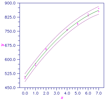
Figure 9, Second Degree Polynomial Fit With 95% One-at-a-Time Prediction Intervals


