RNLIN
Fits a nonlinear regression model.
Required Arguments
FUNC — User-supplied SUBROUTINE to return the weight, frequency, residual, and optionally the derivative of the residual at the given parameter vector THETA for a single observation. The usage is:
CALL FUNC (NPARM, THETA, IOPT, IOBS, FRQ, WT, E, DE, IEND),
where
NPARM – Number of unknown parameters in the regression function. (Input)
THETA – Vector of length NPARM containing parameter values. (Input)
IOPT – Function/derivative evaluation option. (Input)
IOPT | Meaning |
0 | Evaluate the function. |
1 | Evaluate the derivative |
If IDERIV = 0, only IOPT = 0 is used.
IOBS – Observation number. (Input)
The function is evaluated at the IOBS-th observation.
The function is evaluated at the IOBS-th observation.
FRQ – Frequency for the observation. (Output)
WT – Weight for the observation. (Output)
Use WT = 1.0 for equal weighting (unweighted least squares).
Use WT = 1.0 for equal weighting (unweighted least squares).
E – Error (residual) for the IOBS-th observation. (Output, if IOPT = 0)
DE – Vector of length NPARM containing the partial derivatives of the residual for the IOBS-th observation. (Output, if IOPT = 1)
If IDERIV = 0, DE is not referenced and can be a vector of length one.
If IDERIV = 0, DE is not referenced and can be a vector of length one.
IEND – Completion indicator. (Output)
IEND | Meaning |
0 | IOBS is less than or equal to the number of observations. |
1 | IOBS is greater than the number of observations. WT, FRQ, E, and DE are not output. |
FUNC must be declared EXTERNAL in the calling program.
THETA — Vector of length NPARM containing parameter values. (Input/Output)
On input, THETA must contain the initial estimate. On output, THETA contains the final estimate.
On input, THETA must contain the initial estimate. On output, THETA contains the final estimate.
Optional Arguments
NPARM — Number of unknown parameters in the regression function. (Input)
Default: NPARM = size (THETA,1).
Default: NPARM = size (THETA,1).
IDERIV — Derivative option. (Input)
Default: IDERIV = 0.
Default: IDERIV = 0.
IDERIV | Meaning |
0 | Derivatives are obtained by finite differences. |
1 | Derivatives are supplied by FUNC. |
R — NPARM by NPARM upper triangular matrix containing the R matrix from a QR decomposition of the Jacobian. (Output)
LDR — Leading dimension of R exactly as specified in the dimension statement in the calling program. (Input)
Default: LDR = size (R, 1).
Default: LDR = size (R, 1).
IRANK — Rank of R. (Output)
IRANK less than NPARM may indicate the model is overparameterized.
IRANK less than NPARM may indicate the model is overparameterized.
DFE — Degrees of freedom for error. (Output)
SSE — Sums of squares for error. (Output)
FORTRAN 90 Interface
Generic: CALL RNLIN (FUNC, THETA [, …])
Specific: The specific interface names are S_RNLIN and D_RNLIN.
FORTRAN 77 Interface
Single: CALL RNLIN (FUNC, NPARM, IDERIV, THETA, R, LDR, IRANK, DFE, SSE)
Double: The double precision name is DRNLIN.
Description
Routine RNLIN fits a nonlinear regression model using least squares. The nonlinear regression model is
where the observed values of the yi’s constitute the responses or values of the dependent variable, the known xi’s are the vectors of the values of the independent (explanatory) variables, θ is the vector of p regression parameters, and the ɛi’s are independently distributed normal errors with mean zero and variance σ2. For this model, a least squares estimate of θ is also a maximum likelihood estimate of θ.
The residuals for the model are
A value of θ that minimizes
is a least squares estimate of θ. Routine RNLIN is designed so that these residuals are input one at a time from a user-supplied subroutine. This permits RNLIN to handle the case when n is large and the data cannot reside in an array but must reside on some secondary storage device.
Routine RNLIN is based on MINPACK routines LMDIF and LMDER by Moré et al. (1980). The routine RNLIN uses a modified Levenberg-Marquardt method to generate a sequence of approximations to a minimum point. Let
be the current estimate of θ. A new estimate is given by
where sc is a solution to
Here,
is the Jacobian evaluated at
The algorithm uses a “trust region” approach with a step bound of δc. A solution of the equations is first obtained for μc = 0. If ∥sc∥2 < δc, this update is accepted. Otherwise, μc is set to a positive value and another solution is obtained. The method is discussed by Levenberg (1944), Marquardt (1963), and Dennis and Schnabel (1983, pages 129‑147, 218‑338).
If IDERIV = 0, forward finite differences are used to estimate the Jacobian numerically. If IDERIV = 1, the Jacobian is computed analytically via the user-supplied subroutine. With IDERIV = 0 and single precision arithmetic, the estimate of the Jacobian may be so poor that the algorithm terminates at a noncritical point. In such instances, IDERIV = 1 or double precision arithmetic is recommended.
Routine RNLIN does not actually store the Jacobian but uses fast Givens transformations to construct an orthogonal reduction of the Jacobian to upper triangular form (stored in R). The reduction is based on fast Givens transformations (see routines SROTMG and SROTM, Golub and Van Loan 1983, pages 156‑162, Gentleman 1974). This method has two main advantages: (1) the loss of accuracy resulting from forming the crossproduct matrix used in the equations for sc is avoided, and (2) the n × p Jacobian need not be stored saving space when n > p.
A weighted least squares fit can also be performed. This is appropriate when the variance of ɛi in the nonlinear regression model is not constant but instead is σ2/wi. Here, the wi’s are weights input via the user-supplied subroutine. For the weighted case, RNLIN computes a minimum weighted sum of squares for error (stored in SSE).
Comments
1. Workspace may be explicitly provided, if desired, by use of R2LIN/DR2LIN. The reference is:
CALL R2LIN (FUNC, NPARM, IDERIV, THETA, R, LDR, IRANK, DFE, SSE, IPARAM, RPARAM, SCALE, IWK, WK)
The additional arguments are as follows:
IPARAM — Vector of length 6 containing convergence parameters. (Input/Output)
On input, set IPARAM(1) = 0 for default convergence parameter settings. If IPARAM(1) = 0, the remaining elements of IPARAM, and the arguments RPARAM and SCALE need not be initialized.
On input, set IPARAM(1) = 0 for default convergence parameter settings. If IPARAM(1) = 0, the remaining elements of IPARAM, and the arguments RPARAM and SCALE need not be initialized.
I | Name | IPARAM(I) |
|---|---|---|
1 | INIT | Initialization flag. (Input) INIT = 0 means use default settings for IPARAM, RPARAM, and SCALE. INIT = 1 means use the input IPARAM and RPARAM settings. |
2 | NDIGIT | Number of good digits in the residuals. (Input, if IPARAM(1) = 1) |
3 | ITER | Number of iterations. (Input/Output, if IPARAM(1) = 1; Output, otherwise) On input, this is the maximum number of iterations allowed. The default is 100. On output, it is the actual number of iterations. |
4 | NFCN | Number of SSE evaluations. (Input/Output, if IPARAM(1) = 1; Output, if IPARAM(1) = 0) On input, this is the maximum number of evaluations allowed. The default is 400. On output, it is the actual number of evaluations. |
5 | NJAC | Number of Jacobian evaluations. (Input, if IPARAM(1) = 1 and IDERIV = 1; Output, if IDERIV = 1) On input, this is the maximum number of Jacobian evaluations allowed. The default is 100. On output, it is the number of Jacobian evaluations. |
6 | MODE | Scaling option. (Input, if IPARAM(1) = 1) If IPARAM(6) = 1, the values for SCALE are set internally. The default is 1. Otherwise, SCALE must be input. |
RPARAM — Vector of length 7 containing convergence parameters. (Input, if IPARAM(1) = 1)
In the following table, the default settings are given in parentheses. EPS = AMACH(4)(see the documentation for IMSL routine AMACH).
In the following table, the default settings are given in parentheses. EPS = AMACH(4)(see the documentation for IMSL routine AMACH).
I | Name | RPARAM(I) |
|---|---|---|
1 | FJACTL | Scaled gradient tolerance (SQRT(EPS) for single precision; EPS1∕3 for double precision) Convergence is declared if ∣WK(I)∣ * max{∣THETA(I)∣, 1.0/SCALE(I)}/SSE is less than FJACTL for I = 1, 2, …, NPARM, where WK(I) is the I‑th component of the gradient vector. |
2 | STEPTL | Scaled step tolerance (EPS2∕3) Convergence is declared if ∣WK(NPARM + I)∣/max{∣THETA(I)∣, 1.0/SCALE(I)} is less than STEPTL for I = 1, 2, …, NPARM, where WK(NPARM + I) is the I‑th component of the last step. |
3 | RFTOL | Relative function tolerance (max{10−10 EPS2/3} for single precision, max{10−20, EPS2/3} for double precision) Convergence is declared if the change in SSE is less than or equal to RFTOL * SSE in absolute value. |
4 | AFTOL | Absolute function tolerance (max{10−20, EPS2} for single precision; max{10−40, EPS2} for double precision) Convergence is declared if SSE is less than AFTOL. |
5 | FALSTL | False convergence tolerance (100.0 * EPS) |
6 | STEPMX | Maximum allowable step size (1000 * MAX(TOL1, TOL2) where TOL1 = SNRM2(NPARM, SCXTH, 1); TOL2 = SNRM2(NPARM, SCALE, 1) and SCXTH is the elementwise product of SCALE and THETA, i.e., SCXTH(I) = SCALE(I) * THETA(I).) |
7 | DELTA | Size of initial trust region radius (based on the initial scaled Cauchy step) |
SCALE — Vector of length NPARM. (Input/Output, if IPARAM(1) = 1 and IPARAM(6) = 0; Output, if IPARAM(6) = 1)
A common choice is to set all elements of SCALE to 1.0. If good starting values for THETA are known and nonzero, a good choice is SCALE(I) = 1.0/∣THETA(I)∣. Otherwise, for example, if THETA(I) is known to be in the interval (‑105, 105), set SCALE(I) = 10−5. Or, for example, if THETA(I) is known to be in the interval (103, 105), set SCALE(I) = 10−4.
A common choice is to set all elements of SCALE to 1.0. If good starting values for THETA are known and nonzero, a good choice is SCALE(I) = 1.0/∣THETA(I)∣. Otherwise, for example, if THETA(I) is known to be in the interval (‑105, 105), set SCALE(I) = 10−5. Or, for example, if THETA(I) is known to be in the interval (103, 105), set SCALE(I) = 10−4.
IWK — Work vector of length NPARM.
WK — Work vector of length 11 * NPARM + 4. (Output)
The first NPARM components of WK are the gradient at the solution. The second NRARM components of WK give the last step.
The first NPARM components of WK are the gradient at the solution. The second NRARM components of WK give the last step.
2. Informational errors
Type | Code | Description |
|---|---|---|
3 | 1 | Both the scaled actual and predicted reductions in the function are less than or equal to the relative function convergence tolerance. |
3 | 2 | The iterates appear to be converging to a noncritical point. Incorrect gradient information, a discontinuous function, or stopping tolerances being too tight may be the cause. |
4 | 3 | Maximum number of iterations is exceeded. |
4 | 4 | Maximum number of function evaluations is exceeded. |
4 | 5 | Maximum number of Jacobian evaluations is exceeded for IDERIV = 1. |
3 | 6 | Five consecutive steps of the same size have been taken. Either the function is unbounded below, or it has a finite asymptote in some direction, or the stepsize is too small. |
2 | 7 | Scaled step tolerance is satisfied, the current point may be an approximate local solution, or the algorithm is making very slow progress and is not near a solution, or STEPTL is too big. |
3. The first stopping criterion for RNLIN occurs when SSE is less than the absolute function tolerance. The second stopping criterion occurs when the norm of the scaled gradient is less than the given gradient tolerance. The third stopping criterion occurs when the scaled distance between the last two steps is less than the step tolerance. The third stopping criterion also generates error code 7. The fourth stopping criterion occurs when the relative change in SSE is less than RFTOL. The fourth stopping criterion also generates error code 1. See Dennis and Schnabel (1983, pages 159‑161, 278‑280, and 347‑348) for a discussion of stopping criteria and choice of tolerances.
4. To use some nondefault convergence parameters, first call R8LIN, then reset the corresponding convergence parameters to the desired value and call R2LIN. For example, the following code could be used if nondefault convergence parameters are to be used:
!
CALL R8LIN (IPARAM, RPARAM)
! R8LIN outputs IPARAM(1) = 1 to indicate some
! nondefault convergence parameters are to be set.
! R8LIN outputs the remaining elements of IPARAM
! and RPARAM as their default values.
!
! Set some nondefault convergence parameters.
IPARAM(3) = 20
IPARAM(6) = 0
SCALE(1) = 0.1
SCALE(2) = 10.0
!
CALL R2LIN (FUNC, NPARM, IDERIV, THETA, R, &
LDR,IRANK, DFE, SSE, IPARAM, &
RPARAM, SCALE, IWK, WK)
!
CALL R8LIN (IPARAM, RPARAM)
! R8LIN outputs IPARAM(1) = 1 to indicate some
! nondefault convergence parameters are to be set.
! R8LIN outputs the remaining elements of IPARAM
! and RPARAM as their default values.
!
! Set some nondefault convergence parameters.
IPARAM(3) = 20
IPARAM(6) = 0
SCALE(1) = 0.1
SCALE(2) = 10.0
!
CALL R2LIN (FUNC, NPARM, IDERIV, THETA, R, &
LDR,IRANK, DFE, SSE, IPARAM, &
RPARAM, SCALE, IWK, WK)
If double precision is being used, then DR8LIN and DR2LIN are called and RPARAM is declared double precision.
Programming Notes
Nonlinear regression allows substantial flexibility over linear regression because the user can specify the functional form of the model. This added flexibility can cause unexpected convergence problems for users that are unaware of the limitations of the software. Also, in many cases, there are possible remedies that may not be immediatedly obvious. The following is a list of possible convergence problems and some remedies that the user can try. There is not a one-to-one correspondence between the problems and the remedies. Remedies for some problems may also be relevant for the other problems.
1. A local minimum is found. Try a different starting value. Good starting values often can be obtained by fitting simpler models. For example, for a nonlinear function
good starting values can be obtained from the estimated linear regression coefficients

from a simple linear regression of ln y on ln x. The starting values for the nonlinear regression in this case would be
If an approximate linear model is not clear, then simplify the model by reducing the number of nonlinear regression parameters. For example, some nonlinear parameters for which good starting values are known could be set to these values in order to simplify the model for computing starting values for the remaining parameters.
2. The estimate of θ is incorrectly returned as the same or very close to the initial estimate
∙ The scale of the problem may be orders of magnitude smaller than the assumed default of 1 causing premature stopping. For example, in single precision if SSE is less than AMACH(4)**2, the routine stops. See Example 3, which shows how to shut down some of the stopping criteria that may not be relevant for your particular problem and which also shows how to improve the speed of convergence by the input of the scale of the model parameters.
∙ The scale of the problem may be orders of magnitude larger than the assumed default causing premature stopping. The information with regard to the input of the scale of the model parameters in Example 3 is also relevant here. In addition, the maximum allowable step size, RPARAM(6) in Example 3, may need to be increased.
∙ The residuals are input with accuracy much less than machine accuracy causing premature stopping because a local minimum is found. Again see Example 3 to see generally how to change some default tolerances. If you cannot improve the precision of the computations of the residual, you need to set IPARAM(2) to indicate the actual number of good digits in the residuals.
3. The model is discontinuous as a function of θ. You may have a mistake in the subroutine you supplied. Note that the function f(x; θ) can be a discontinuous function of x.
4. The R matrix returned by RNLIN is inaccurate. Use the double precision version DRNLIN. If IDERIV = 1, check your derivatives or try using IDERIV = 0. If IDERIV = 0, try using IDERIV = 1.
5. Overflow occurs during the computations. Print out θ and the residual in the subroutine you supplied. Make sure the code you supply does not overflow at some value of θ.
6. The estimate of θ is going to infinity. You may need to reparameterize or change your function. For example, a parameterization in terms of the reciprocals may be appropriate.
7. Some components of θ are outside known bounds. Routine RNLIN does not handle bounds on the parameters, but you can artificially impose some by setting the residuals unusually large outside the bounds. Although this introduces a discontinuity in the model function, this often works and allows you to use RNLIN without having to resort to a more general nonlinear optimization routine.
Examples
Example 1
This example uses data discussed by Neter, Wasserman, and Kutner (1983, pages 475‑478). A nonlinear model
is fitted. The option IDERIV = 0 is used.
The user must supply a SUBROUTINE to return the residual, weight, and frequency for a single observation at the given value of the regression parameter vector θ. This subroutine, called EXAMPL here, must be declared EXTERNAL in the calling program and must have the specified calling sequence.
USE RNLIN_INT
USE UMACH_INT
USE WRRRN_INT
IMPLICIT NONE
INTEGER LDR, NOBS, NPARM
PARAMETER (NOBS=15, NPARM=2, LDR=NPARM)
!
INTEGER IRANK, NOUT
REAL DFE, R(LDR,NPARM), SSE, THETA(NPARM)
EXTERNAL EXAMPL
!
DATA THETA/60.0, -0.03/
!
CALL UMACH (2, NOUT)
!
CALL RNLIN (EXAMPL, THETA, r=r, irank=irank, dfe=dfe, sse=sse)
WRITE (NOUT,*) 'THETA = ', THETA
WRITE (NOUT,*) 'IRANK = ', IRANK, ' DFE = ', DFE, ' SSE = ', &
SSE
CALL WRRRN ('R', R)
END
!
SUBROUTINE EXAMPL (NPARM, THETA, IOPT, IOBS, FRQ, WT, E, DE, &
IEND)
INTEGER NPARM, IOPT, IOBS, IEND
REAL THETA(NPARM), FRQ, WT, E, DE(1)
!
INTEGER NOBS
PARAMETER (NOBS=15)
!
REAL EXP, XDATA(NOBS), YDATA(NOBS)
INTRINSIC EXP
!
DATA YDATA/54.0, 50.0, 45.0, 37.0, 35.0, 25.0, 20.0, 16.0, 18.0, &
13.0, 8.0, 11.0, 8.0, 4.0, 6.0/
DATA XDATA/2.0, 5.0, 7.0, 10.0, 14.0, 19.0, 26.0, 31.0, 34.0, &
38.0, 45.0, 52.0, 53.0, 60.0, 65.0/
!
IF (IOBS .LE. NOBS) THEN
WT = 1.0E0
FRQ = 1.0E0
IEND = 0
E = YDATA(IOBS) - THETA(1)*EXP(THETA(2)*XDATA(IOBS))
ELSE
IEND = 1
END IF
RETURN
END
Output
THETA = 58.6045 -3.95835E-02
IRANK = 2 DFE = 13.0000 SSE = 49.4593
R
1 2
1 1.9 1139.8
2 0.0 1139.7
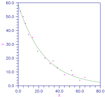
Figure 10, Plot of the Nonlinear Fit
Example 2
This example fits the model in Example 1 with the option IDERIV = 1.
USE RNLIN_INT
USE UMACH_INT
USE WRRRN_INT
IMPLICIT NONE
INTEGER LDR, NOBS, NPARM
PARAMETER (NOBS=15, NPARM=2, LDR=NPARM)
!
INTEGER IDERIV, IRANK, NOUT
REAL DFE, R(LDR,NPARM), SSE, THETA(NPARM)
EXTERNAL EXAMPL
!
DATA THETA/60.0, -0.03/
!
CALL UMACH (2, NOUT)
!
IDERIV = 1
CALL RNLIN (EXAMPL, THETA, IDERIV=IDERIV, r=r, irank=irank, dfe=dfe, &
sse=sse)
WRITE (NOUT,*) 'THETA = ', THETA
WRITE (NOUT,*) 'IRANK = ', IRANK, ' DFE = ', DFE, ' SSE = ', &
SSE
CALL WRRRN ('R', R)
END
!
SUBROUTINE EXAMPL (NPARM, THETA, IOPT, IOBS, FRQ, WT, E, DE, &
IEND)
INTEGER NPARM, IOPT, IOBS, IEND
REAL THETA(NPARM), FRQ, WT, E, DE(NPARM)
!
INTEGER NOBS
PARAMETER (NOBS=15)
!
REAL EXP, XDATA(NOBS), YDATA(NOBS)
INTRINSIC EXP
!
DATA YDATA/54.0, 50.0, 45.0, 37.0, 35.0, 25.0, 20.0, 16.0, 18.0, &
13.0, 8.0, 11.0, 8.0, 4.0, 6.0/
DATA XDATA/2.0, 5.0, 7.0, 10.0, 14.0, 19.0, 26.0, 31.0, 34.0, &
38.0, 45.0, 52.0, 53.0, 60.0, 65.0/
!
IF (IOBS .LE. NOBS) THEN
WT = 1.0E0
FRQ = 1.0E0
IEND = 0
IF (IOPT .EQ. 0) THEN
E = YDATA(IOBS) - THETA(1)*EXP(THETA(2)*XDATA(IOBS))
ELSE
DE(1) = -EXP(THETA(2)*XDATA(IOBS))
DE(2) = -THETA(1)*XDATA(IOBS)*EXP(THETA(2)*XDATA(IOBS))
END IF
ELSE
IEND = 1
END IF
RETURN
END
Output
THETA = 58.6034 -3.95812E-02
IRANK = 2 DFE = 13.0000 SSE = 49.4593
R
1 2
1 1.9 1140.1
2 0.0 1139.9
Example 3
This example fits the model in Example 1, but the data for y is 10−10 times the values in Example 1. In order to solve this problem without rescaling y, we use some nondefault convergence tolerances and scales. This is accomplished by invoking routine R8LIN, setting some elements of IPARAM, RPARAM, and SCALE, and then invoking R2LIN. Here, we set the absolute function tolerance to 0.0. The default value would cause the program to terminate after one iteration because the residual sum of squares is roughly 10−19 Also, we set the relative function tolerance to 0.0. The gradient stopping condition is properly scaled for this problem so we leave it at its default value. Finally, we set SCALE(I) equal to the absolute value of the reciprocal of the starting value.
Note in the output that the estimate of θ1 is 10−10 times the estimate in Example 1. Note also that the invocation of R2LIN in place of RNLIN allows the printing of additional information that is output in IPARAM (number iterations and number of SSE evaluations) and output in WK (gradient at solution and last step).
USE UMACH_INT
USE R8LIN_INT
USE R2LIN_INT
USE WROPT_INT
USE WRRRN_INT
IMPLICIT NONE
INTEGER LDR, NOBS, NPARM, IDERIV, ISETNG
PARAMETER (NOBS=15, NPARM=2, LDR=NPARM)
!
INTEGER IPARAM(6), IRANK, IWK(NPARM), NOUT
REAL ABS, DFE, R(LDR,NPARM), RPARAM(7), SCALE(NPARM), SSE, &
THETA(NPARM), WK(11*NPARM+4)
INTRINSIC ABS
EXTERNAL EXAMPL
!
DATA THETA/6.0E-9, -0.03/
!
CALL UMACH (2, NOUT)
!
CALL R8LIN (IPARAM, RPARAM)
RPARAM(3) = 0.0
RPARAM(4) = 0.0
IPARAM(6) = 0
SCALE(1) = 1.0/ABS(THETA(1))
SCALE(2) = 1.0/ABS(THETA(2))
CALL R2LIN (EXAMPL, NPARM, IDERIV, THETA, R, LDR, IRANK, DFE, &
SSE, IPARAM, RPARAM, SCALE, IWK, WK)
WRITE (NOUT,*) 'THETA = ', THETA
WRITE (NOUT,*) 'IRANK = ', IRANK, ' DFE = ', DFE, ' SSE = ', &
SSE
WRITE (NOUT,*) 'Number of iterations = ', IPARAM(3)
WRITE (NOUT,*) 'Number of SSE evaluations = ', IPARAM(4)
ISETNG=2
CALL WROPT (-6, ISETNG, 1)
CALL WRRRN ('Gradient at solution', WK, 1, NPARM, 1)
CALL WRRRN ('Last step taken', WK((NPARM+1):), 1, NPARM, 1)
CALL WRRRN ('R', R)
END
!
SUBROUTINE EXAMPL (NPARM, THETA, IOPT, IOBS, FRQ, WT, E, DE, &
IEND)
INTEGER NPARM, IOPT, IOBS, IEND
REAL THETA(NPARM), FRQ, WT, E, DE(1)
!
INTEGER NOBS
PARAMETER (NOBS=15)
!
REAL EXP, XDATA(NOBS), YDATA(NOBS)
INTRINSIC EXP
!
DATA YDATA/54.0E-10, 50.0E-10, 45.0E-10, 37.0E-10, 35.0E-10, &
25.0E-10, 20.0E-10, 16.0E-10, 18.0E-10, 13.0E-10, 8.0E-10, &
11.0E-10, 8.0E-10, 4.0E-10, 6.0E-10/
DATA XDATA/2.0, 5.0, 7.0, 10.0, 14.0, 19.0, 26.0, 31.0, 34.0, &
38.0, 45.0, 52.0, 53.0, 60.0, 65.0/
!
IF (IOBS .LE. NOBS) THEN
WT = 1.0E0
FRQ = 1.0E0
IEND = 0
E = YDATA(IOBS) - THETA(1)*EXP(THETA(2)*XDATA(IOBS))
ELSE
IEND = 1
END IF
RETURN
END
Output
THETA = 5.86076E-09 -3.95879E-02
RANK = 2 DFE = 13.0000 SSE = 4.94593E-19
Number of iterations = 5
Number of SSE evaluations = 13
Gradient at solution
1 2
6.86656E-14 -1.73762E-20
Last step taken
1 2
-3.24588E-14 3.65805E-07
R
1 2
1 1.87392E+00 1.13981E-07
2 0.00000E+00 1.13934E-07
Example 4
For an extended version of Example 2 that in addition computes the estimated asymptotic variance-covariance matrix of the estimated nonlinear regression parameters, see Example 2 for routine RCOVB. The example also computes confidence intervals for the parameters.
Example 5


