SEASONAL_FIT
Estimates the optimum differencing for a non‑stationary time series using an autoregressive model, AR(p), to adjust the series for seasonality.
Required Arguments
Z — Vector containing the time series. (Input)
MAXLAG — Maximum lag allowed when fitting an AR(p) model,
1 <= MAXLAG <= NOBSZ/2. (Input)
1 <= MAXLAG <= NOBSZ/2. (Input)
IPERA — NDIFF by nipera matrix containing the seasonal differences to test. (Input)
Here, nipera = SIZE(IPERA, 2) must be greater than or equal to one.
All elements of IPERA must be greater than or equal to one.
Here, nipera = SIZE(IPERA, 2) must be greater than or equal to one.
All elements of IPERA must be greater than or equal to one.
W — Allocatable array which, on return, will contain the differenced series. (Output)
Optional Arguments
NOBSZ— Number of observations in time series Z. (Input)
Default: NOBSZ = SIZE(Z).
Default: NOBSZ = SIZE(Z).
NDIFF — Number of differences to use. (Input)
NDIFF must be greater than or equal to one.
Default: NDIFF = SIZE(IPERA, 1).
NDIFF must be greater than or equal to one.
Default: NDIFF = SIZE(IPERA, 1).
IORDA — NDIFF by niorda matrix containing the possible orders of each difference given in IPERA. (Input)
Here, niorda = SIZE(IORDA, 2) must be greater than or equal to one.
All elements of IORDA must be non‑negative.
Default: IORDA is an NDIFF by 1 matrix, where IORDA (1:NDIFF, 1) =1.
Here, niorda = SIZE(IORDA, 2) must be greater than or equal to one.
All elements of IORDA must be non‑negative.
Default: IORDA is an NDIFF by 1 matrix, where IORDA (1:NDIFF, 1) =1.
IMISS — Missing value option. (Input)
Default: IMISS = 0
Default: IMISS = 0
IMISS | Action |
|---|---|
0 | Include missing values in W. |
1 | Exclude missing values from W. |
NOBSW — Number of observations in the differenced series W. (Output)
NOBSW = NOBSZ ‑ IMISS * NLOST
NOBSW = NOBSZ ‑ IMISS * NLOST
NLOST — Number of observations lost because of differencing the time series Z. (Output)
IOPT_PERA — Vector of length NDIFF containing the column from matrix IPERA which produced the differenced series represented in W. (Output)
IOPT_ORDA — Vector of length NDIFF containing the column from matrix IORDA which produced the differenced series represented in W. (Output)
NPAR — The optimum value for the autoregressive lag. (Output)
AIC — Akaike's Information Criterion (AIC) for the optimum seasonally adjusted model. (Output)
FORTRAN 90 Interface
Generic: CALL SEASONAL_FIT (Z, MAXLAG, IPERA, W [, …])
Specific: The specific interface names are S_SEASONAL_FIT and D_SEASONAL_FIT.
Description
Many time series contain seasonal trends and cycles that can be modeled by first differencing the series. For example, if the correlation is strong from one period to the next, the series might be differenced by a lag of 1. Instead of fitting a model to the series , the model is fitted to the transformed series: . Higher order lags or differences are warranted if the series has, for example, a cycle every 4 or 13 weeks.
Routine SEASONAL_FIT does not center the original series. For every combination of columns in IPERA and IORDA, the series is converted to the seasonally adjusted series using the following computation
where s:= (s1,… ,sm) , d:= (d1,… ,dm) represent specific columns of arrays IPERA and IORDA respectively, and m = NDIFF.
This transformation of the series to is accomplished using routine DIFF. After this transformation, a call is made to AUTO_UNI_AR to automatically determine the optimum lag for an AR(p) representation for . This procedure is repeated for every possible combination of columns of IPERA and IORDA. The series with the minimum AIC is identified as the optimum representation and returned in vector W.
Example
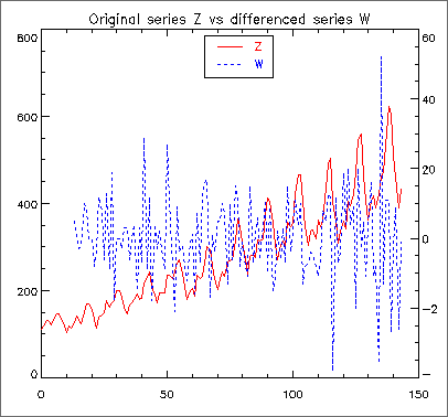
Consider the Airline Data (Box, Jenkins and Reinsel 1994, p. 547) consisting of the monthly total number of international airline passengers from January 1949 through December 1960. Routine SEASONAL_FIT is used to compute the optimum seasonality representation of the adjusted series
where or and
A differenced series with minimum AIC,
Note: The numerical output may be viewed by removing the comments from the WRITE statement lines in the following example. |
USE GDATA_INT
USE SEASONAL_FIT_INT
IMPLICIT NONE
integer :: nout
integer, parameter :: nobs = 144, ndiff = 2, maxlag = 10
integer :: nlost, npar, i
integer :: NROW, NCOL
real, dimension(144,1) :: z
real :: aic
integer, dimension(2,2) :: ipera
integer :: nobsw
real, dimension(:), allocatable :: w
integer, dimension(ndiff) :: iopt_pera, iopt_orda
ipera(1,1) = 1; ipera(1,2) = 1
ipera(2,1) = 1; ipera(2,2) = 12
CALL GDATA (4, z, NROW, NCOL)
CALL seasonal_fit(z(:,1), maxlag, ipera, w, NDIFF = ndiff, NLOST = nlost, &
IOPT_PERA = iopt_pera, NOBSW = nobsw, &
IOPT_ORDA = iopt_orda, NPAR = npar, AIC = aic)
CALL UMACH(2,nout)
! WRITE (nout,*) "nlost =", nlost
! WRITE (nout,*) "iopt_pera = (", iopt_pera(1),",", iopt_pera(2), ")"
! WRITE (nout,*) "iopt_orda = (", iopt_orda(1),",", iopt_orda(2), ")"
! WRITE (nout,*) "Order of optimum AR process: ", npar
! WRITE (nout,*) "aic =", aic
! WRITE (nout,*) " "
! WRITE (nout,*) "Size of w:", nobsw
! WRITE (nout,*) "i z(i,1) w(i)"
! DO i=1,nobs
! WRITE (nout,*) i, z(i,1), w(i)
! END DO
IF (ALLOCATED(w)) DEALLOCATE(w)
END PROGRAM
Output

Figure 15, Differenced Series


