PACF
Computes the sample partial autocorrelation function of a stationary time series.
Required Arguments
MAXLAG — Maximum lag of partial autocorrelations to be computed. (Input)
AC — Vector of length MAXLAG+ 1 containing the autocorrelations of the time series X. (Input)
AC(0) = 1. AC(k) contains the autocorrelation of lag k where k = 1, …, MAXLAG.
AC(0) = 1. AC(k) contains the autocorrelation of lag k where k = 1, …, MAXLAG.
PAC — Vector of length MAXLAG containing the partial autocorrelations of the time series X. (Output)
The partial autocorrelation of lag k corresponds to PAC(k) where k = 1, …, MAXLAG.
The partial autocorrelation of lag k corresponds to PAC(k) where k = 1, …, MAXLAG.
FORTRAN 90 Interface
Generic: CALL PACF (MAXLAG, AC, PAC)
Specific: The specific interface names are S_PACF and D_PACF.
FORTRAN 77 Interface
Single: CALL PACF (MAXLAG, AC, PAC)
Double: The double precision name is DPACF.
Description
Routine PACF estimates the partial autocorrelations of a stationary time series given the
K = MAXLAG sample autocorrelations
K = MAXLAG sample autocorrelations
for k = 0, 1, …, K. Consider the AR(k) process defined by
where ɸkj denotes the j‑th coefficient in the process. The set of estimates
for k = 1, …, K is the sample partial autocorrelation function. The autoregressive parameters
for j = 1, …, k are approximated by Yule‑Walker estimates for successive AR(k) models where k = 1, …, K. Based on the sample Yule‑Walker equations
a recursive relationship for k = 1, …, K was developed by Durbin (1960). The equations are given by
and
This procedure is sensitive to rounding error and should not be used if the parameters are near the nonstationarity boundary. A possible alternative would be to estimate { ɸkk} for successive AR(k) models using least squares (IMSL routine NSLSE) or maximum likelihood. Based on the hypothesis that the true process is AR(p), Box and Jenkins (1976, page 65) note
See Box and Jenkins (1976, pages 82–84) for more information concerning the partial autocorrelation function.
Comments
Workspace may be explicitly provided, if desired, by use of P2CF/DP2CF. The reference is:
CALL P2CF (MAXLAG, AC, PAC, WK)
The additional argument is:
WK — Work vector of length 2 * MAXLAG.
Example
Consider the Wolfer Sunspot Data (Anderson 1971, page 660) consisting of the number of sunspots observed each year from 1749 through 1924. The data set for this example consists of the number of sunspots observed from 1770 through 1869. Routine PACF to used to compute the estimated partial autocorrelations.
USE GDATA_INT
USE ACF_INT
USE PACF_INT
USE WRRRL_INT
IMPLICIT NONE
INTEGER IMEAN, IPRINT, ISEOPT, MAXLAG, NOBS
PARAMETER (IMEAN=1, IPRINT=0, ISEOPT=0, MAXLAG=20, NOBS=100)
!
INTEGER NCOL, NROW
REAL AC(0:MAXLAG), ACV(0:MAXLAG), PAC(MAXLAG), &
RDATA(176,2), SEAC(1), X(NOBS), XMEAN
CHARACTER CLABEL(2)*4, RLABEL(1)*6
!
EQUIVALENCE (X(1), RDATA(22,2))
!
DATA RLABEL/'NUMBER'/, CLABEL/'Lag ', 'PACF'/
! Wolfer Sunspot Data for
! years 1770 through 1869
CALL GDATA (2, RDATA, NROW, NCOL)
! Compute sample ACF
CALL ACF (X, MAXLAG, AC)
! Compute sample PACF
CALL PACF (MAXLAG, AC, PAC)
! Print results
CALL WRRRL (' ', PAC, RLABEL, CLABEL, FMT= '(F8.3)')
!
END
Output
Lag PACF
1 0.806
2 -0.635
3 0.078
4 -0.059
5 -0.001
6 0.172
7 0.109
8 0.110
9 0.079
10 0.079
11 0.069
12 -0.038
13 0.081
14 0.033
15 -0.035
16 -0.131
17 -0.155
18 -0.119
19 -0.016
20 -0.004
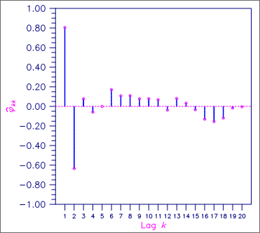
Figure 17, Sample Partial Autocorrelation Function


