Notation that is consistently used throughout this chapter is given in the following table. The FORTRAN equivalent of the symbols used are also given.

The routines in this chapter can generally be used for one or more of several purposes. Among these purposes are the following:

The idea in principal components is to find a small number of linear combinations of the original variables that maximize the variance accounted for in the original data. This amounts to an eigensystem analysis of the covariance (or correlation) matrix. In addition to the eigensystem analysis, routine PRINC computes standard errors for the eigenvalues. Correlations of the original variables with the principal component scores are also computed.

The computation of common principal components via routine KPRIN is equivalent to finding the “eigenvectors” that best simultaneously diagonalize one or more variance‑covariance matrices. For only one input variance‑covariance matrix, the vectors computed actually are the eigenvectors of the matrix.

Factor analysis and principal component analysis, while quite different in assumptions, often serve the same ends. Unlike principal components in which linear combinations yielding the highest possible variances are obtained, factor analysis generally obtains linear combinations of the observed variables according to a model relating the observed variables to hypothesized underlying factors, plus a random error term called the unique error or uniqueness. In factor analysis, the unique errors associated with each variable are usually assumed to be independent of the factors. In addition, in the common factor model, the unique errors are assumed to be mutually independent. The factor analysis model is

where x is the p vector of observed variables, μ is the p vector of variable means, Λ is the p × k matrix of factor loadings, f is the k vector of hypothesized underlying random factors, and e is the p vector of hypothesized unique random errors.

Because much of the computation in factor analysis was originally done by hand or was expensive on early computers, quick (but dirty) algorithms that made the calculations possible were developed. One result is the many factor extraction methods available today. Generally speaking, in the exploratory or model building phase of a factor analysis, a method of factor extraction that is not computationally intensive (such as principal components, principal factor, or image analysis) is used. If desired, a computationally intensive method is then used to obtain (what is hoped will be) the final factors.

In exploratory factor analysis, the unrotated factor loadings obtained from the factor extraction are generally transformed (rotated) to simplify the interpretation of the factors. Rotation is possible because of the overparameterization in the factor analysis model. The method used for rotation may result in factors that are independent (orthogonal rotations) or correlated (oblique rotations). Prior information may be available (or hypothesized) in which case a Procrustes rotation could be used. When no prior information is available, an analytic rotation can be performed.

Once the factor loadings have been extracted and rotated (if desired), estimates for the hypothesized underlying factors can be computed. First, one of several available methods in routine FCOEF is used to compute the factor score coefficients. Routine FSCOR is then called with these factor score coefficients to compute the factor scores.

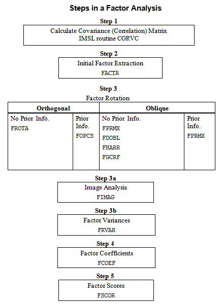
The steps generally used in a factor analysis are summarized as follows:

Routine MVIND computes the Wilks likelihood‑ratio test of independence among several sets of variables. Routines CANCR and CANVC compute some other tests of independence between exactly two sets of variables. Routine CANCR uses the raw data as input while CANVC uses the sample variance‑covariance matrix. Furthermore, CANCR and CANVC perform a canonical correlation analysis. Since CANCR uses a better algorithm in terms of numerical stability (it does not compute the covariance matrix), CANCR should be used if possible. However, if the raw data is not available, or if there is too much data for all of it to reside in memory at the same time, or if multiple canonical correlation analyses are to be performed based on the same pre‑computed sample variance‑covariance matrix, then the use of CANVC may be necessary. Canonical correlation analysis is useful for characterizing the independent linear statistical relationships that exist between the two sets of variables. This involves computing linear combinations of the variables in the two separate sets and their associated correlation. The coefficients of the variables in the linear combinations are called the “canonical coefficients,” and the correlations are called “canonical correlations.” Evaluation of the linear combinations using the canonical coefficients gives the “canonical scores.” Routine CANCR computes the canonical scores for the observed data. Routine FSCOR can be used to compute the canonical scores for new data or for the observed data if CANVC is used.