.ix.

Chapter 10: Linear Algebra Operators and Generic Functions

.ix.

Computes the product of the inverse of a matrix and a vector or matrix.

Operator Return Value

Matrix containing the product of A^-1 and B. (Output)

Required Operands

A — Left operand matrix. This is an array of rank 2, or 3. It may be real, double, complex, double complex, or one of the computational sparse matrix derived types, ?_hbc_sparse. (Input)

B — Right operand matrix or vector. This is an array of rank 1, 2, or 3. It may be real, double, complex, or double complex. (Input)

Optional Variables, Reserved Names

This operator uses the routines lin_sol_gen or lin_sol_lsq (See Chapter 1, “Linear Systems”).

The option and derived type names are given in the following tables:

Option Names for .ix.	Option Value
use_lin_sol_gen_only	1
use_lin_sol_lsq_only	2
ix_options_for_lin_sol_gen	3
ix_options_for_lin_sol_lsq	4
Skip_error_processing	5

Name of Unallocated Option Array to Use for Setting Options	Use	Derived Type
?_invx_options(:)	Use when setting options for calls hereafter.	?_options
?_invx_options_once(:)	Use when setting options for next call only.	?_options

For a description on how to use these options, see Matrix Optional Data Changes. See lin_sol_gen and lin_sol_lsq located in Chapter 1, “Linear Systems” for the specific options for these routines.

FORTRAN 90 Interface

A .ix. B

Description

Computes the product of the inverse of matrix A and vector or matrix B, for square non-singular matrices or the corresponding Moore-Penrose generalized inverse matrix for singular square matrices or rectangular matrices. The operation may be read generalized inverse times. The results are in a precision and data type that matches the most accurate or complex operand.

.ix. can be used with either dense or sparse matrices. It is MPI capable for dense matrices only.

Examples

Dense Matrix Example (operator_ex01.f90)

use linear_operators

implicit none

! This is the equivalent of Example 1 for LIN_SOL_GEN, with operators
! and functions.

integer, parameter :: n=32

real(kind(1e0)) :: one=1.0e0, err

real(kind(1e0)), dimension(n,n) :: A, b, x

! Generate random matrices for A and b:

A = rand(A); b=rand(b)

! Compute the solution matrix of Ax = b.

x = A .ix. b

! Check the results.

err = norm(b - (A .x. x))/(norm(A)*norm(x)+norm(b))

if (err <= sqrt(epsilon(one))) &

write (*,*) 'Example 1 for LIN_SOL_GEN (operators) is correct.'

end

Sparse Matrix Example 1

use wrrrn_int

use linear_operators

type (s_sparse) S

type (s_hbc_sparse) H

integer, parameter :: N=3

real (kind(1.e0)) x(N,N), y(N,N), B(N,N)

real (kind(1.e0)) err

S = s_entry (1, 1, 2.0)

S = s_entry (1, 3, 1.0)

S = s_entry (2, 2, 4.0)

S = s_entry (3, 3, 6.0)

H = S ! sparse

X = H ! dense equivalent of H

B= rand(B)

Y = H .ix. B

call wrrrn ( 'H', X)

call wrrrn ( 'B', b)

call wrrrn ( 'H .ix. B ', y)

! Check the results.

err = norm(y - (X .ix. B))

if (err <= sqrt(epsilon(one))) then

write (*,*) 'Sparse example for .ix. operator is correct.'

end if

end

Output

1 2 3

1 2.000 0.000 1.000

2 0.000 4.000 0.000

3 0.000 0.000 6.000

1 2 3

1 0.8292 0.5697 0.1687

2 0.9670 0.7296 0.0603

3 0.1458 0.2726 0.8809

H .ix. B

1 2 3

1 0.4025 0.2621 0.0109

2 0.2417 0.1824 0.0151

3 0.0243 0.0454 0.1468

Sparse Matrix Example 2: Plane Poisson Problem with Dirichlet Boundary Conditions

We want to calculate a numerical solution, which approximates the true solution of the Poisson (boundary value) problem in the solution domain, a rectangle in The equation is

There are Dirichlet boundary conditions on

There are further Neumann boundary conditions on

The boundary arcs comprisingare mutually exclusive of each other. The functions are defined on their respective domains.

We will solve an instance of this problem by using finite differences to approximate the derivatives. This will lead to a sparse system of linear algebraic equations. Note that particular cases of this problem can be solved with methods that are likely to be more efficient or more appropriate than the one illustrated here. We use this method to illustrate our matrix data handling routines and defined operators.

The area of the rectangleis with the origin fixed at the lower left or SW corner. The dimension along the axis isand along theaxis is. A rectangular uniform grid is defined on where each sub-rectangle in the grid has sides and. What is perhaps novel in our development is that the boundary values are written into the linear system as trivial equations. This leads to more unknowns than standard approaches to this problem but the complexity of describing the equations into computer code is reduced. The boundary conditions are naturally in place when the solution is obtained. No reshaping is required.

We number the approximate values ofat the grid points and collapse them into a single vector. Given a coordinate of the grid, we use the mappingto define coordinateof this vector. This mapping enables us to define the matrix that is used to solve for the values ofat the grid points.

For the Neumann boundary conditions we taketo be the East face of the rectangle. Along that edge we have, and we impose the smooth interface.

Our use of finite differences is standard. For the differential equation we approximate

at the inner grid points . For the Neumann condition we approximate

The remaining equations come from the Dirichlet conditions given on.

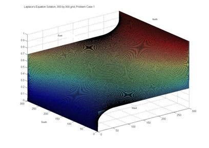
To illustrate three examples of solutions to this problem we consider

1. A Laplace Equation with the boundary conditions
          , on the South Edge
          , on the East Edge
          , on the North Edge
          , on the West Edge
The functionfor all. Graphical results are shown below with the title Problem Case 1

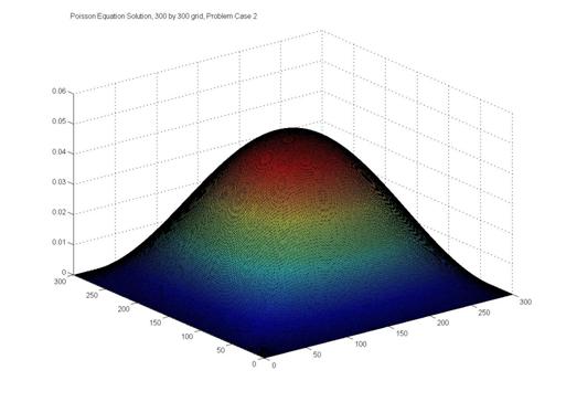
2. A Poisson equation with the boundary conditions on all of the edges and . This problem has the solution, and this identity provides a way of verifying that the accuracy is within the truncation error implied by the difference equations. Graphical results are shown with the title Problem Case 2 The residual function verifies the expected accuracy.

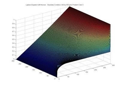
3. The Laplace Equation with the boundary conditions of Problem Case 1 except that the boundary condition on the East Edge is replaced by the Neumann condition. Graphical results are shown as Problem Case 3.”

Subroutine document_ex2

! Illustrate a 2D Poisson equation with Dirichlet and

! Neumann boundary conditions.

! These modules defines the structures and overloaded assignment code.

Use linear_operators

Implicit None

Integer :: I, J, JJ, MY_CASE, IFILE

Integer, Parameter :: N = 300, M = 300

Real (Kind(1.d0)) :: a = 1.d0, b = 1.d0

Real (Kind(1.d0)) :: delx, dely, r, s, pi, scale

Real (Kind(1.d0)) :: u(N*M), w(N*M), P(N, M)

Real (Kind(1.e0)) :: TS, TE

CHARACTER(LEN=12) :: PR_LABEL(3)=&

(/'Laplace','Poisson','Neumann'/)

! Mapping function (in-line) for grid coordinate to

! matrix-vector indexing.

JJ (I, J) = I + (J-1) * N

! Define sparse matrices to hold problem data.

Type (d_sparse) C

Type (d_hbc_sparse) D

! Define differences and related parameters.

delx = a / (N-1)

dely = b / (M-1)

r = 1.d0 / delx ** 2

s = 1.d0 / dely ** 2

Do MY_CASE = 1, 3

! For MY_CASE =

! 1. Solve boundary value problem with f=0 and Dirichlet

! boundary conditions.

! 2. Solve Poisson equation with f such that a solution is known.

! Use zero boundary condtions.

! 3. Solve boundary value problem with Dirichlet condtions as in 1.

! except on the East edge. There the partial WRT x is zero.

! Set timer for building the matrix.

Call cpu_time (TS)

Do I = 2, N - 1

Do J = 2, M - 1

! Write entries for second partials WRT x and y.

C = d_entry (JJ(I, J), JJ(I-1, J), r)

C = d_entry (JJ(I, J), JJ(I+1, J), r)

C = d_entry (JJ(I, J), JJ(I, J),-2*(r+s))

C = d_entry (JJ(I, J), JJ(I, J-1), s)

C = d_entry (JJ(I, J), JJ(I, J+1), s)

! Define components of the right-hand side.

w (JJ(I, J)) = f((I-1)*delx, (J-1)*dely, MY_CASE)

End Do

! Write entries for Dirichlet boundary conditions.

! First do the South edge, then the West, then the North.

Select Case (MY_CASE)

Case (1:2)

Do I = 1, N

C = d_entry (JJ(I, 1), JJ(I, 1), r+s)

w (JJ(I, 1)) = g ((I-1)*delx, 0.d0, MY_CASE) * (r+s)

End Do

Do J = 2, M - 1

C = d_entry (JJ(1, J), JJ(1, J), r+s)

w (JJ(1, J)) = g (0.d0, (J-1)*dely, MY_CASE) * (r+s)

End Do

Do I = 1, N

C = d_entry (JJ(I, M), JJ(I, M), r+s)

w (JJ(I, M)) = g ((I-1)*delx, b, MY_CASE) * (r+s)

End Do

Do J = 2, M - 1

C = d_entry (JJ(N, J), JJ(N, J), (r+s))

w (JJ(N, J)) = g (a, (J-1)*dely, MY_CASE) * (r+s)

End Do

Case (3)

! Write entries for the boundary values but avoid the East edge.

Do I = 1, N - 1

C = d_entry (JJ(I, 1), JJ(I, 1), r+s)

w (JJ(I, 1)) = g ((I-1)*delx, 0.d0, MY_CASE) * (r+s)

End Do

Do J = 2, M - 1

C = d_entry (JJ(1, J), JJ(1, J), r+s)

w (JJ(1, J)) = g (0.d0, (J-1)*dely, MY_CASE) * (r+s)

End Do

Do I = 1, N - 1

C = d_entry (JJ(I, M), JJ(I, M), r+s)

w (JJ(I, M)) = g ((I-1)*delx, b, MY_CASE) * (r+s)

End Do

! Write entries for the Neumann condition on the East edge.

Do J = 1, M

C = d_entry (JJ(N, J), JJ(N, J), 1.d0/delx)

C = d_entry (JJ(N, J), JJ(N-2, J),-1.d0/delx)

w (JJ(N, J)) = 0.d0

End Do

End Select

! Convert to Harwell-Boeing format for solving.

D = C

Call cpu_time (TE)

Write (*,'(A,F6.2," S. - ",A)') "Time to build matrix = ", &

TE - TS, PR_LABEL(MY_CASE)

! Clear sparse triplets.

C = 0

! Turn off iterative refinement for maximal performance.

! This is generally not recommended unless

! the problem is known not to require it.

If (MY_CASE == 2) D%options%iterRefine = 0

! This is the solve step.

Call cpu_time (TS)

u = D .ix. w

Call cpu_time (TE)

Write (*,'(A,I6," is",F6.2," S")') &

"Time to solve system of size = ", N * M, TE - TS

! This is a second solve step using the factorization

! from the first step.

Call cpu_time (TS)

u = D .ix. w

Call cpu_time (TE)

If(MY_CASE == 1) then

Write (*,'(A,I6," is",F6.2," S")') &

"Time for a 2nd system of size (iterative refinement) =", &

N * M, TE - TS

Else

Write (*,'(A,I6," is",F6.2," S")') &

"Time for a 2nd system of size (without refinement) =", &

N * M, TE - TS

End if

! Convert solution vector to a 2D array of values.

P = reshape (u , (/ N, M /))

If (MY_CASE == 2) Then

pi = dconst ('pi')

scale = - 0.5 / pi ** 2

Do I = 1, N

Do J = 1, M

! This uses the known form of the solution to compute residuals.

P (I, J) = P (I, J) - scale * f ((I-1)*delx, &

(J-1)*dely, MY_CASE)

End Do

write (*,*) minval (P), " = min solution error "

write (*,*) maxval (P), " = max solution error "

End If

Write (*,'(A,1pE12.4/)') "Condition number of matrix", cond (D)

! Clear all matrix data for next problem case.

D = 0

End Do ! MY_CASE

Contains

Function f (x, y, MY_CASE)

implicit none

! Define the right-hand side function associated with the

! "del" operator.

Real (Kind(1.d0)) x, y, f, pi

Integer MY_CASE

if(MY_CASE == 2) THEN

pi = dconst ('pi')

f = - Sin (pi*x) * Sin (pi*y)

Else

f = 0.d0

End If

End Function

Function g (x, y, MY_CASE)

implicit none

! Define the edge values, except along East edge, x = a.

Real (Kind(1.d0)) x, y, g

Integer MY_CASE

! Fill in a constant value along each edge.

If (MY_CASE == 1 .Or. MY_CASE == 3) Then

If (y == 0.d0) Then

g = 0.d0

Return

End If

If (y == b) Then

g = 1.d0

Return

End If

If (x == 0.d0) Then

g = 0.3d0

Return

End If

If (x == a) Then

g = 0.7d0

End If

Else

g = 0.d0

End If

End Function

End Subroutine

Problem Case 1

Problem Case 2

Problem Case 3

Parallel Example (parallel_ex01.f90)

use linear_operators

use mpi_setup_int

implicit none

! This is the equivalent of Parallel Example 1 for .ix., with box data types

! and functions.

integer, parameter :: n=32, nr=4

real(kind(1e0)) :: one=1e0

real(kind(1e0)), dimension(n,n,nr) :: A, b, x, err(nr)

! Setup for MPI.

MP_NPROCS=MP_SETUP()

! Generate random matrices for A and b:

A = rand(A); b=rand(b)

! Compute the box solution matrix of Ax = b.

x = A .ix. b

! Check the results.

err = norm(b - (A .x. x))/(norm(A)*norm(x)+norm(b))

if (ALL(err <= sqrt(epsilon(one))) .and. MP_RANK == 0) &

write (*,*) 'Parallel Example 1 is correct.'

! See to any error messages and quit MPI.

MP_NPROCS=MP_SETUP('Final')

end

Visual Numerics, Inc.
Visual Numerics - Developers of IMSL and PV-WAVE
http://www.vni.com/
PHONE: 713.784.3131
FAX:713.781.9260