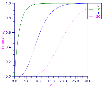
This function evaluates the chi-squared cumulative distribution function.

Function Return Value

CHIDF — Function value, the probability that a chi-squared random variable takes a value less than or equal to CHSQ.   (Output)

Required Arguments

CHSQ — Argument for which the chi-squared distribution function is to be evaluated.   (Input)

DF — Number of degrees of freedom of the chi-squared distribution.   (Input)
DF must be positive.

Optional Arguments

COMPLEMENT — Logical. If .TRUE., the complement of the chi-squared cumulative distribution function is evaluated.  If .FALSE., the chi-squared cumulative distribution function is evaluated.   (Input)
See the Description section for further details on the use of COMPLEMENT.
Default: COMPLEMENT = .FALSE..

FORTRAN 90 Interface

Generic:                              CHIDF (CHSQ, DF [,…])

Specific:                             The specific interface names are S_CHIDF and D_CHIDF.

FORTRAN 77 Interface

Single:                                CHIDF (CHSQ, DF)

Double:                              The double precision name is DCHIDF.

Description

Function CHIDF evaluates the cumulative distribution function, F, of a chi-squared random variable with DF degrees of freedom, that is, with v = DF, and x = CHSQ,

 

where Γ(⋅) is the gamma function. The value of the distribution function at the point x is the probability that the random variable takes a value less than or equal to x.

For v > vmax = {343 for double precision, 171 for single precision}, CHIDF uses the Wilson-Hilferty approximation (Abramowitz and Stegun [A&S] 1964, equation 26.4.17) for p in terms of the normal CDF, which is evaluated using function ANORDF. 

For v ≤ vmax , CHIDF uses series expansions to evaluate p: for x < ν, CHIDF calculates p using A&S series 6.5.29, and for x  > ν, CHIDF calculates p using the continued fraction expansion of the incomplete gamma function given in A&S equation 6.5.31.

If COMPLEMENT = .TRUE., the value of CHIDF at the point x is 1− p, where 1− p is the probability that the random variable takes a value greater than x. In those situations where the desired end result is 1− p, the user can achieve greater accuracy in the right tail region by using the result returned by CHIDF with the optional argument COMPLEMENT set to .TRUE. rather than by using
1− p where p is the result returned by CHIDF with COMPLEMENT set to .FALSE..

Figure 11- 8   Chi-Squared Distribution Function

Comments

Informational errors

Type Code

1         1                  Since the input argument, CHSQ, is less than zero, the distribution function is zero at CHSQ.

2         3                  The normal distribution is used for large degrees of freedom. However, it has produced underflow. Therefore, the probability, CHIDF, is set to zero.

Example

Suppose X is a chi-squared random variable with 2 degrees of freedom. In this example, we find the probability that X is less than 0.15 and the probability that X is greater than 3.0.

 

      USE CHIDF_INT

      USE UMACH_INT

      IMPLICIT   NONE

 

      INTEGER    NOUT

      REAL       CHSQ, DF, P

 

      CALL UMACH (2, NOUT)

      DF   = 2.0

      CHSQ = 0.15

      P    = CHIDF(CHSQ,DF)

      WRITE (NOUT,99998) P

99998 FORMAT (' The probability that chi-squared with 2 df is less ', &

            'than 0.15 is ', F6.4)

      CHSQ = 3.0

      P    = CHIDF(CHSQ,DF, complement=.true.)

      WRITE (NOUT,99999) P

99999 FORMAT (' The probability that chi-squared with 2 df is greater ' &

            , 'than 3.0 is ', F6.4)

      END

Output

 

  The probability that chi-squared with 2 df is less than 0.15 is 0.0723

  The probability that chi-squared with 2 df is greater than 3.0 is 0.2231

 

http://www.vni.com/ PHONE: 713.784.3131 FAX:713.781.9260