Cdf (JMSL Numerical Library)

Overview

Package

Class

Tree

Index

Help

JMSL^TM Numerical Library 6.0

PREV CLASS NEXT CLASS

FRAMES NO FRAMES

SUMMARY: NESTED | FIELD | CONSTR | METHOD

DETAIL: FIELD | CONSTR | METHOD

com.imsl.stat
Class Cdf

java.lang.Object
  com.imsl.stat.Cdf

public final class Cdf
extends Object
extends Object

Cumulative probability distribution functions.

See Also:: Example, Probability density function, Inverse Cumulative Distribution Function

Method Summary
`static double`	`beta(double x, double pin, double qin)` Evaluates the beta cumulative probability distribution function.
`static double`	`betaMean(double pin, double qin)` Evaluates the mean of the beta cumulative probability distribution function
`static double`	`betaVariance(double pin, double qin)` Evaluates the variance of the beta cumulative probability distribution function
`static double`	`binomial(int k, int n, double pin)` Evaluates the binomial cumulative probability distribution function.
`static double`	`bivariateNormal(double x, double y, double rho)` Evaluates the bivariate normal cumulative probability distribution function.
`static double`	`chi(double chsq, double df)` Evaluates the chi-squared cumulative distribution function (CDF).
`static double`	`chiMean(double df)` Evaluates the mean of the chi-squared cumulative probability distribution function
`static double`	`chiVariance(double df)` Evaluates the variance of the chi-squared cumulative probability distribution function
`static double`	`complementaryChi(double chsq, double df)` Calculates the complement of the chi-squared cumulative distribution function.
`static double`	`complementaryF(double x, double dfn, double dfd)` Calculates the complement of the F distribution function.
`static double`	`complementaryStudentsT(double t, double df)` Calculates the complement of the Student's t distribution.
`static double`	`discreteUniform(int x, int n)` Evaluates the discrete uniform cumulative probability distribution function.
`static double`	`exponential(double x, double scale)` Evaluates the exponential cumulative probability distribution function.
`static double`	`extremeValue(double x, double mu, double beta)` Evaluates the extreme value cumulative probability distribution function.
`static double`	`F(double x, double dfn, double dfd)` Evaluates the F cumulative probability distribution function.
`static double`	`gamma(double x, double a)` Evaluates the gamma cumulative probability distribution function.
`static double`	`geometric(int x, double pin)` Evaluates the discrete geometric cumulative probability distribution function.
`static double`	`hypergeometric(int k, int sampleSize, int defectivesInLot, int lotSize)` Evaluates the hypergeometric cumulative probability distribution function.
`static double`	`logistic(double x, double mu, double s)` Evaluates the logistic cumulative probability distribution function.
`static double`	`logNormal(double x, double mu, double sigma)` Evaluates the standard lognormal cumulative probability distribution function.
`static double`	`noncentralBeta(double x, double shape1, double shape2, double lambda)` Evaluates the noncentral beta cumulative distribution function (CDF).
`static double`	`noncentralchi(double chsq, double df, double alam)` Evaluates the noncentral chi-squared cumulative probability distribution function.
`static double`	`noncentralF(double f, double df1, double df2, double lambda)` Evaluates the noncentral F cumulative distribution function (CDF).
`static double`	`noncentralstudentsT(double t, int idf, double delta)` Evaluates the noncentral Student's t cumulative probability distribution function.
`static double`	`normal(double x)` Evaluates the normal (Gaussian) cumulative probability distribution function.
`static double`	`Pareto(double x, double xm, double k)` Evaluates the Pareto cumulative probability distribution function.
`static double`	`poisson(int k, double theta)` Evaluates the Poisson cumulative probability distribution function.
`static double`	`Rayleigh(double x, double alpha)` Evaluates the Rayleigh cumulative probability distribution function.
`static double`	`studentsT(double t, double df)` Evaluates the Student's t cumulative probability distribution function.
`static double`	`uniform(double x, double aa, double bb)` Evaluates the uniform cumulative probability distribution function.
`static double`	`Weibull(double x, double gamma, double alpha)` Evaluates the Weibull cumulative probability distribution function.

Methods inherited from class java.lang.Object
`clone, equals, finalize, getClass, hashCode, notify, notifyAll, toString, wait, wait, wait`

Method Detail

beta

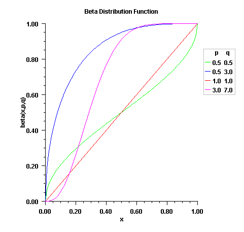
public static double beta(double x,
                          double pin,
                          double qin)

Evaluates the beta cumulative probability distribution function.

Method beta evaluates the distribution function of a beta random variable with parameters pin and qin. This function is sometimes called the incomplete beta ratio and, with p = pin and q = qin, is denoted by . It is given by

$I_x left( {p,,q} right) = frac{{Gamma left( p right)Gamma left( q right)}}{{Gamma left( {p + q} right)}}int_0^x {,t^{p - 1} left( {1 - t} right)^{q - 1} dt}$

where is the gamma function. The value of the distribution function is the probability that the random variable takes a value less than or equal to x.

The integral in the expression above is called the incomplete beta function and is denoted by . The constant in the expression is the reciprocal of the beta function (the incomplete function evaluated at one) and is denoted by .

beta uses the method of Bosten and Battiste (1974).

Plot of Beta Distribution Function

Parameters:: x - a double, the argument at which the function is to be evaluated.; pin - a double, the first beta distribution parameter.; qin - a double, the second beta distribution parameter.
Returns:: a double, the probability that a beta random variable takes on a value less than or equal to x.
See Also:: Example

betaMean

public static double betaMean(double pin,
                              double qin)

Evaluates the mean of the beta cumulative probability distribution function

Parameters:: pin - a double, the first beta distribution parameter.; qin - a double, the second beta distribution parameter.
Returns:: a double, the mean of the beta distribution function.

betaVariance

public static double betaVariance(double pin,
                                  double qin)

Evaluates the variance of the beta cumulative probability distribution function

Parameters:: pin - a double, the first beta distribution parameter.; qin - a double, the second beta distribution parameter.
Returns:: a double, the variance of the beta distribution function.

binomial

public static double binomial(int k,
                              int n,
                              double pin)

Evaluates the binomial cumulative probability distribution function.

Method binomial evaluates the distribution function of a binomial random variable with parameters n and p with p=pin. It does this by summing probabilities of the random variable taking on the specific values in its range. These probabilities are computed by the recursive relationship

$Pr left( {X = j} right) = frac{{left( {n + 1 - j} right)p}}{{jleft( {1 - p} right)}}Pr left( {X = j - 1} right)$

To avoid the possibility of underflow, the probabilities are computed forward from 0, if k is not greater than n times p, and are computed backward from n, otherwise. The smallest positive machine number, , is used as the starting value for summing the probabilities, which are rescaled by if forward computation is performed and by if backward computation is done. For the special case of p = 0, binomial is set to 1; and for the case p = 1, binomial is set to 1 if k = n and to 0 otherwise.

Parameters:: k - the int argument for which the binomial distribution function is to be evaluated.; n - the int number of Bernoulli trials.; pin - a double scalar value representing the probability of success on each independent trial.
Returns:: a double scalar value representing the probability that a binomial random variable takes a value less than or equal to k. This value is the probability that k or fewer successes occur in n independent Bernoulli trials, each of which has a pin probability of success.
See Also:: Example

bivariateNormal

public static double bivariateNormal(double x,
                                     double y,
                                     double rho)

Evaluates the bivariate normal cumulative probability distribution function. Let

be a bivariate normal variable with mean

and variance-covariance matrix

$left[ begin{array}{cc} 1 & rho \ rho & 1end{array}right]$

This method computes the probability that

and

Plot of Bivariate Normal Distribution Function

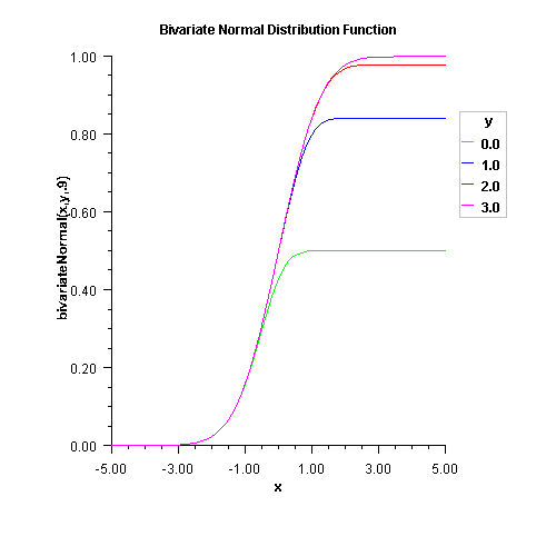
Parameters:: x - is the x-coordinate of the point for which the bivariate normal distribution function is to be evaluated.; y - is the y-coordinate of the point for which the bivariate normal distribution function is to be evaluated.; rho - is the correlation coefficient.
Returns:: the probability that a bivariate normal random variable with correlation rho satisfies and .

chi

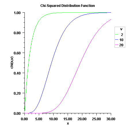
public static double chi(double chsq,
                         double df)

Evaluates the chi-squared cumulative distribution function (CDF).

Method chi evaluates the cumulative distribution function (CDF) F, of a chi-squared random variable with df degrees of freedom, that is, with x = chsq and = df,

$Fleft( x, nu right) ;=; frac{1}{{2^{nu /2} Gamma left( {nu /2} right)}} int_0^x {e^{ - t/2} t^{nu /2 - 1} } dt$

where is the gamma function. The value is the probability that the random variable takes a value less than or equal to x.

For , chi uses the Wilson-Hilferty approximation (Abramowitz and Stegun [A&S] 1964, equation 26.4.17) for p in terms of the normal CDF, which is evaluated using method normal.

For , chi uses series expansions to evaluate p. chi first uses the A&S series 6.5.29 to calculate p, but if and $x ;ge; max(frac{nu}{2}, ;2)$ , chi recalculates p. If or , chi uses a continued fraction expansion (A&S equation 6.5.31) to calculate p, otherwise an asymptotic expansion (A&S equation 6.5.32) is used.

For greater right tail accuracy, see complementaryChi(double, double).

Plot of Chi-Squared Distribution Function

Parameters:: chsq - a double scalar value representing the argument at which the function is to be evaluated.; df - a double scalar value representing the number of degrees of freedom. df must be positive.
Returns:: a double scalar value representing the probability that a chi-squared random variable takes a value less than or equal to chsq.
See Also:: Example

chiMean

public static double chiMean(double df)

Evaluates the mean of the chi-squared cumulative probability distribution function

Parameters:: df - a double scalar value representing the number of degrees of freedom. This must be at least 0.5.
Returns:: a double, the mean of the chi-squared distribution function.

chiVariance

public static double chiVariance(double df)

Evaluates the variance of the chi-squared cumulative probability distribution function

Parameters:: df - a double scalar value representing the number of degrees of freedom. This must be at least 0.5.
Returns:: a double, the variance of the chi-squared distribution function.

complementaryChi

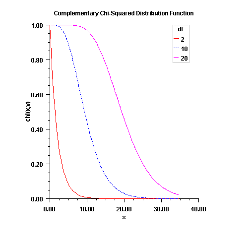
public static double complementaryChi(double chsq,
                                      double df)

Calculates the complement of the chi-squared cumulative distribution function.

Method complementaryChi evaluates the cumulative distribution function, , of a chi-squared random variable with df degrees of freedom, that is, with x = chsq and = df,

$p ;=; Fleft( x, nu right) ;=; frac{1}{{2^{nu /2} Gamma left( {nu /2} right)}} int_0^x {e^{ - t/2} t^{nu /2 - 1} } dt$

where is the gamma function. The value of the complementaryChi distribution function at the point x, , is the probability that the random variable takes a value greater than x.

For , complementaryChi uses the Wilson-Hilferty approximation (Abramowitz and Stegun [A&S] 1964, equation 26.4.17) for p in terms of the normal CDF, which is evaluated using method normal.

For , complementaryChi uses series expansions to evaluate p. complementaryChi first uses the A&S series 6.5.29 to calculate p, but if and $x ;ge; max(frac{nu}{2}, ;2)$ , complementaryChi recalculates p. If or , complementaryChi uses a continued fraction expansion (A&S equation 6.5.31) to calculate p, otherwise an asymptotic expansion (A&S equation 6.5.32) is used.

complementaryChi provides greater right tail accuracy for the Chi-squared distribution than does 1 - chi.

Plot of Chi-Squared Distribution Function

Parameters:: chsq - a double scalar value at which the function is to be evaluated.; df - a double scalar value representing the number of degrees of freedom. df must be positive.
Returns:: a double scalar value representing the probability that a chi-squared random variable takes a value greater than chsq.

complementaryF

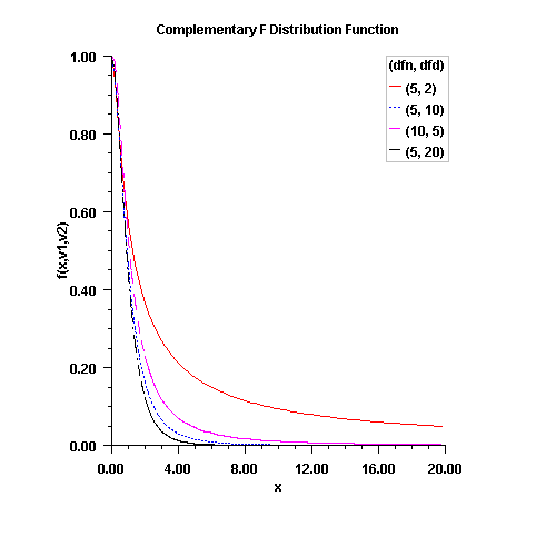
public static double complementaryF(double x,
                                    double dfn,
                                    double dfd)

Calculates the complement of the F distribution function.

complementaryF evaluates one minus the distribution function of a Snedecor's F random variable with dfn numerator degrees of freedom and dfd denominator degrees of freedom. The function is evaluated by making a transformation to a beta random variable and then using the function beta. If X is an F variate with and degrees of freedom and , then Y is a beta variate with parameters and . complementaryF also uses a relationship between F random variables that can be expressed as follows:

This function provides higher right tail accuracy for the F distribution.

Plot of F Distribution Function

Parameters:: x - a double, the argument at which is to be evaluated.; dfn - a double, the numerator degrees of freedom. It must be positive.; dfd - a double, the denominator degrees of freedom. It must be positive.
Returns:: a double, the probability that an F random variable takes on a value greater than x.

complementaryStudentsT

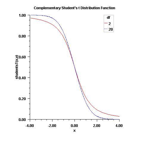
public static double complementaryStudentsT(double t,
                                            double df)

Calculates the complement of the Student's t distribution.

Method complementaryStudentsT evaluates one minus the distribution function of a Student's t random variable with df degrees of freedom. If the square of t is greater than or equal to df, the relationship of a t to an f random variable (and subsequently, to a beta random variable) is exploited, and routine beta is used. Otherwise, the method described by Hill (1970) is used. If df is not an integer, if df is greater than 19, or if df is greater than 200, a Cornish-Fisher expansion is used to evaluate the distribution function. If df is less than 20 and is less than 2.0, a trigonometric series (see Abramowitz and Stegun 1964, equations 26.7.3 and 26.7.4, with some rearrangement) is used. For the remaining cases, a series given by Hill (1970) that converges well for large values of t is used.

This function provides higher right tail accuracy for the Student's t distribution.

complementary Student's t Distribution Function

Parameters:: t - a double scalar value for which is to be evaluated; df - a double scalar value representing the number of degrees of freedom. This must be at least one.
Returns:: a double scalar value representing the probability that a Student's t random variable takes a value greater than t.
See Also:: Example

discreteUniform

public static double discreteUniform(int x,
                                     int n)

Evaluates the discrete uniform cumulative probability distribution function.

Parameters:: x - an int scalar value representing the argument at which the function is to be evaluated. x should be a value between the lower limit 0 and upper limit n; n - an int scalar value representing the upper limit of the discrete uniform distribution.
Returns:: a double scalar value representing the probability that a discrete uniform random variable takes a value less than or equal to x.

exponential

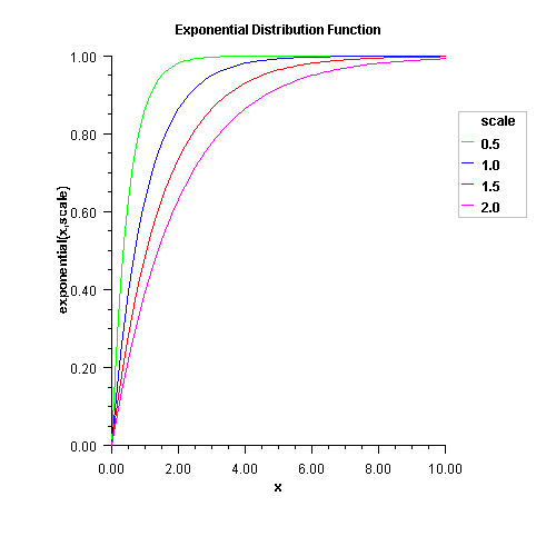
public static double exponential(double x,
                                 double scale)

Evaluates the exponential cumulative probability distribution function.

Method exponential is a special case of the gamma distribution function, which evaluates the distribution function, F, with scale parameter b and shape parameter a, used in the gamma distribution function equal to 1.0. That is,

$Fleft( x right) = frac{1}{{Gamma left( a right)}}int_0^x {e^{ - t/b}} dt$

where is the gamma function. (The gamma function is the integral from 0 to of the same integrand as above). The value of the distribution function at the point x is the probability that the random variable takes a value less than or equal to x.

If x is less than or equal to 1.0, gamma uses a series expansion. Otherwise, a continued fraction expansion is used. (See Abramowitz and Stegun, 1964.)

Plot of Exponential Distribution Function

Parameters:: x - a double scalar value representing the argument at which the function is to be evaluated.; scale - a double scalar value representing the scale parameter, .
Returns:: a double scalar value representing the probability that an exponential random variable takes on a value less than or equal to x.
See Also:: Example

extremeValue

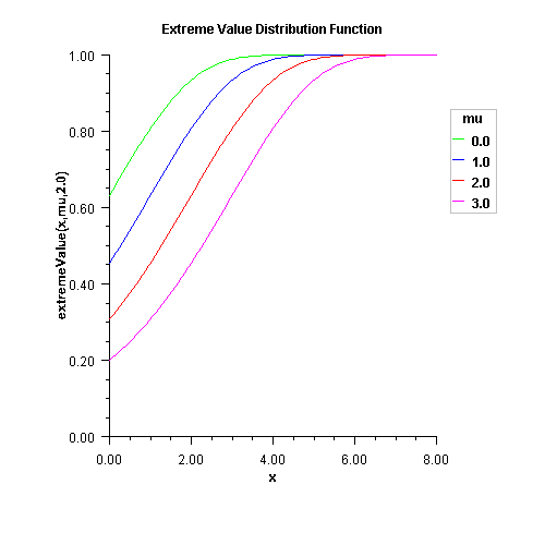
public static double extremeValue(double x,
                                  double mu,
                                  double beta)

Evaluates the extreme value cumulative probability distribution function.

Method extremeValue, also known as the Gumbel minimum distribution, evaluates the extreme value distribution function, F, of a uniform random variable with location parameter and shape parameter ; that is,

$Fleft( x right) = int_0^x {1 - e^{ - e^{frac{x-mu}{beta}}}} dt$

The case where and is called the standard Gumbel distribution.

Random numbers are generated by evaluating uniform variates , equating the continuous distribution function, and then solving for by first computing $frac{x_i - mu}{beta}=log(-log(1-u_i))$ .

Plot of Extreme Value Distribution Function

Parameters:: x - a double scalar value representing the argument at which the function is to be evaluated.; mu - a double scalar value representing the location parameter, .; beta - a double scalar value representing the scale parameter,
Returns:: a double scalar value representing the probability that an extreme value random variable takes on a value less than or equal to x.
See Also:: Example

F

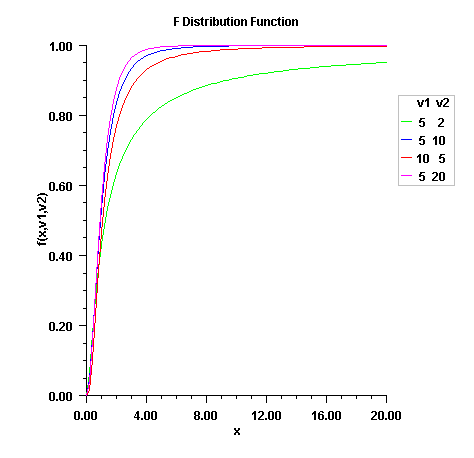
public static double F(double x,
                       double dfn,
                       double dfd)

Evaluates the F cumulative probability distribution function.

F evaluates the distribution function of a Snedecor's F random variable with dfn numerator degrees of freedom and dfd denominator degrees of freedom. The function is evaluated by making a transformation to a beta random variable and then using the function beta. If X is an F variate with and degrees of freedom and , then Y is a beta variate with parameters and . F also uses a relationship between F random variables that can be expressed as follows:

For greater right tail accuracy, see complementaryF(double, double, double).

Plot of F Distribution Function

Parameters:: x - a double, the argument at which the function is to be evaluated.; dfn - a double, the numerator degrees of freedom. It must be positive.; dfd - a double, the denominator degrees of freedom. It must be positive.
Returns:: a double, the probability that an F random variable takes on a value less than or equal to x.
See Also:: Example

gamma

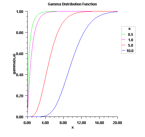
public static double gamma(double x,
                           double a)

Evaluates the gamma cumulative probability distribution function.

Method gamma evaluates the distribution function, F, of a gamma random variable with shape parameter a; that is,

$Fleft( x right) = frac{1}{{Gamma left( a right)}}int_0^x {e^{ - t} t^{a - 1} } dt$

The gamma distribution is often defined as a two-parameter distribution with a scale parameter b (which must be positive), or even as a three-parameter distribution in which the third parameter c is a location parameter. In the most general case, the probability density function over is

$fleft( t right) = frac{1}{{b^a Gamma left( a right)}}e^{ - left( {t - c} right)/b} left( {x - c} right)^{a - 1}$

If T is such a random variable with parameters a, b, and c, the probability that can be obtained from gamma by setting .

If X is less than a or if X is less than or equal to 1.0, gamma uses a series expansion. Otherwise, a continued fraction expansion is used. (See Abramowitz and Stegun, 1964.)

Gamma Distribution Function

Parameters:: x - a double scalar value representing the argument at which the function is to be evaluated.; a - a double scalar value representing the shape parameter. This must be positive.
Returns:: a double scalar value representing the probability that a gamma random variable takes on a value less than or equal to x.
See Also:: Example

geometric

public static double geometric(int x,
                               double pin)

Evaluates the discrete geometric cumulative probability distribution function.

Parameters:: x - an int scalar value representing the argument at which the function is to be evaluated; pin - an double scalar value representing the probability parameter for each independent trial (the probability of success for each independent trial).
Returns:: a double scalar value representing the probability that a geometric random variable takes a value less than or equal to x. The return value is the probability that up to x trials would be observed before observing a success.

hypergeometric

public static double hypergeometric(int k,
                                    int sampleSize,
                                    int defectivesInLot,
                                    int lotSize)

Evaluates the hypergeometric cumulative probability distribution function.

Method hypergeometric evaluates the distribution function of a hypergeometric random variable with parameters n, l, and m. The hypergeometric random variable X can be thought of as the number of items of a given type in a random sample of size n that is drawn without replacement from a population of size l containing m items of this type. The probability function is

$Pr left( {X = j} right) = frac{{left( {_j^m } right)left( {_{n - j}^{l - m} } right)}}{{left( {_n^l } right)}}{rm{for }},,j = i,;i + 1,,,i + 2,; ldots ,;min left( {n,m} right)$

where .

If k is greater than or equal to i and less than or equal to , hypergeometric sums the terms in this expression for j going from i up to k. Otherwise, hypergeometric returns 0 or 1, as appropriate. So, as to avoid rounding in the accumulation, hypergeometric performs the summation differently depending on whether or not k is greater than the mode of the distribution, which is the greatest integer less than or equal to .

Parameters:: k - an int, the argument at which the function is to be evaluated.; sampleSize - an int, the sample size, n.; defectivesInLot - an int, the number of defectives in the lot, m.; lotSize - an int, the lot size, l.
Returns:: a double, the probability that a hypergeometric random variable takes a value less than or equal to k.
See Also:: Example

logistic

public static double logistic(double x,
                              double mu,
                              double s)

Evaluates the logistic cumulative probability distribution function.

Method logistic evaluates the distribution function, F, of a logistic random variable with location parameter and scale parameter s. It is given by

$F(x,mu,s)=frac{1}{1+e^{-(x-mu)/s}}$

where .

Parameters:: x - a double scalar value representing the argument at which the function is to be evaluated.; mu - a double scalar value representing the location parameter, .; s - a double scalar value representing the scale parameter.
Returns:: a double scalar value representing the probability that a logistic random variable takes a value less than or equal to x.

logNormal

public static double logNormal(double x,
                               double mu,
                               double sigma)

Evaluates the standard lognormal cumulative probability distribution function.

$Fleft( x right) = frac{1}{x^{sigma}sqrt{2pi}} int{frac{1}{t}e^{-frac{ {ln{t}-mu}^2 }{2{sigma}^2}} }$

Plot of Lognormal Distribution Function

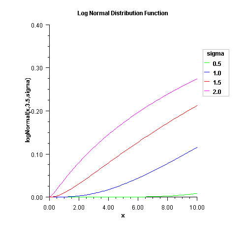
Parameters:: x - a double scalar value representing the argument at which the function is to be evaluated.; mu - a double scalar value representing the location parameter.; sigma - a double scalar value representing the shape parameter. sigma must be a positive.
Returns:: a double scalar value representing the probability that a standard lognormal random variable takes a value less than or equal to x.

noncentralBeta

public static double noncentralBeta(double x,
                                    double shape1,
                                    double shape2,
                                    double lambda)

Evaluates the noncentral beta cumulative distribution function (CDF).

The noncentral beta distribution is a generalization of the beta distribution. If is a noncentral chi-square random variable with noncentrality parameter and degrees of freedom, and is a chi-square random variable with degrees of freedom which is statistically independent of , then

$X ;; = ;; frac{Z}{Z ; + ; Y} ;; = ;; frac{alpha_1 F}{alpha_1 F ; + ; alpha_2}$

is a noncentral beta-distributed random variable and

$F ;; = ;; frac{alpha_2 Z}{alpha_1 Y} ;; = ;; frac{alpha_2 X}{alpha_1 (1 ; - ; X)}$

is a noncentral F-distributed random variable. The CDF for noncentral beta variable X can thus be simply defined in terms of the noncentral F CDF:

$CDF_{ncbeta}(x, ; alpha_1, ; alpha_2, ; lambda) ;; = ;; CDF_{ncF}(f, ; 2 alpha_1, ; 2 alpha_2, ; lambda)$

where $CDF_{ncbeta}(x, ; alpha_1, ; alpha_2, ; lambda)$ is the noncentral beta CDF with = x, = shape1, = shape2, and noncentrality parameter = lambda; $CDF_{ncF}(f, ; 2 alpha_1, ; 2 alpha_2, ; lambda)$ is the noncentral F CDF with argument f, numerator and denominator degrees of freedom and respectively, and noncentrality parameter ; and:

$f ;; = ;; frac{alpha_2 x}{alpha_1 (1 ; - ; x)}; ;; x ;; = ;; frac{alpha_1 f}{alpha_1 f ; + ; alpha_2}$

(See documentation for class Cdf method noncentralF for a discussion of how the noncentral F CDF is defined and calculated.)

With a noncentrality parameter of zero, the noncentral beta distribution is the same as the beta distribution.

Parameters:: x - a double scalar value representing the argument at which the function is to be evaluated. x must be nonnegative and less than or equal to 1.; shape1 - a double scalar value representing the first shape parameter. shape1 must be positive.; shape2 - a double scalar value representing the second shape parameter. shape2 must be positive.; lambda - a double scalar value representing the noncentrality parameter. lambda must nonnegative.
Returns:: a double scalar value representing the probability that a noncentral beta random variable takes a value less than or equal to x.

noncentralchi

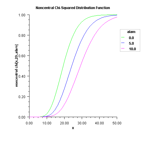
public static double noncentralchi(double chsq,
                                   double df,
                                   double alam)

Evaluates the noncentral chi-squared cumulative probability distribution function.

Method noncentralchi evaluates the distribution function, F, of a noncentral chi-squared random variable with df degrees of freedom and noncentrality parameter alam, that is, with , , and ,

$Fleft( x right) = sumlimits_{i = 0}^infty {frac{e^{-lambda/2}left(lambda/2right)^i}{i!}} int_0^x {frac{t^{left(nu + 2iright)/2-1}e^{ - t/2}} {2^{left(nu+2iright)/2}{Gammaleft(frac{nu+2i}{2}right)}}} dt$

where is the gamma function. This is a series of central chi-squared distribution functions with Poisson weights. The value of the distribution function at the point x is the probability that the random variable takes a value less than or equal to x.

The noncentral chi-squared random variable can be defined by the distribution function above, or alternatively and equivalently, as the sum of squares of independent normal random variables. If the have independent normal distributions with means ${mu}_i$ and variances equal to one and

$X = sumlimits_{i = 1}^n{Y_i}^2$

then has a noncentral chi-squared distribution with degrees of freedom and noncentrality parameter equal to

$sumlimits_{i = 1}^n{mu_i}^2$

With a noncentrality parameter of zero, the noncentral chi-squared distribution is the same as the chi-squared distribution.

noncentralchi determines the point at which the Poisson weight is greatest, and then sums forward and backward from that point, terminating when the additional terms are sufficiently small or when a maximum of 1000 terms have been accumulated. The recurrence relation 26.4.8 of Abramowitz and Stegun (1964) is used to speed the evaluation of the central chi-squared distribution functions.

Noncentral Chi-Squared Distribution Function

Parameters:: chsq - a double scalar value representing the argument at which the function is to be evaluated.; df - a double scalar value representing the number of degrees of freedom. df must be positive.; alam - a double scalar value representing the noncentrality parameter. This must be nonnegative, and alam + df must be less than or equal to 200,000.
Returns:: a double scalar value representing the probability that a chi-squared random variable takes a value less than or equal to chsq.
See Also:: Example

noncentralF

public static double noncentralF(double f,
                                 double df1,
                                 double df2,
                                 double lambda)

Evaluates the noncentral F cumulative distribution function (CDF).

The noncentral F distribution is a generalization of the F distribution. If is a noncentral chi-square random variable with noncentrality parameter and degrees of freedom, and is a chi-square random variable with degrees of freedom which is statistically independent of , then

$F ;; = ;; frac{ (X/nu_1)}{(Y/nu_2)}$

is a noncentral F-distributed random variable whose CDF is given by:

$CDF(f, nu_1, nu_2, lambda) ;; = ;; int_0^f {PDF(x, nu_1, nu_2, lambda)dx}$

where the probability density function is given by:

$PDF(x, nu_1, nu_2, lambda) ;; = ;; Psi ; sum_{k = 0}^infty {Phi_k}$

where

$Psi ;; = ;; frac{ e^{-lambda/2}(nu_1 x)^{nu_1/2}(nu_2)^{nu_2/2} } { x ; (nu_1 x ; + ; nu_2)^{(nu_1 + nu_2)/2} ; Gamma(nu_2/2) }$

$Phi_k ;; = ;; frac{ R^k ; Gamma(frac{nu_1 + nu_2}{2} ; + ; k) } { k! ; Gamma(frac{nu_1}{2} ; + ; k) }$

$R ;; = ;; frac{ lambda nu_1 x }{ 2 (nu_1 x ; + ; nu_2)}$

and

is the gamma function,

= df1,

= df2,

= lambda, and f = f.

With a noncentrality parameter of zero, the noncentral F distribution is the same as the F distribution.

Parameters:: f - a double value representing the argument at which the function is to be evaluated. f must be nonnegative.; df1 - a double value representing the number of numerator degrees of freedom. df1 must be positive.; df2 - a double value representing the number of denominator degrees of freedom. df2 must be positive.; lambda - a double value representing the noncentrality parameter. lambda must be nonnegative.
Returns:: a double scalar value representing the probability that a noncentral F random variable takes a value less than or equal to f.

noncentralstudentsT

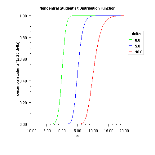
public static double noncentralstudentsT(double t,
                                         int idf,
                                         double delta)

Evaluates the noncentral Student's t cumulative probability distribution function.

Method noncentralstudentsT evaluates the distribution function F of a noncentral t random variable with idf degrees of freedom and noncentrality parameter delta; that is, with , , and $t_{0}= t$ ,

$F{left({t_0}right)} = int_{-{infty}}^{t_{0}} {frac {nu^{nu/2}e^{{-delta^2}/2}} {{sqrt{pi}Gammaleft(nu/2right)left(nu+x^2right)}^{left(nu+1right)/2}} } sumlimits_{i = 0}^infty {Gammaleft(left(nu+i+1right)/2right)left(frac{delta^i}{i!}right)left(frac{2x^2}{nu+x^2}right)^{i/2} dx }$

where is the gamma function. The value of the distribution function at the point $t_{0}$ is the probability that the random variable takes a value less than or equal to $t_{0}$ .

The noncentral t random variable can be defined by the distribution function above, or alternatively and equivalently, as the ratio of a normal random variable and an independent chi-squared random variable. If w has a normal distribution with mean and variance equal to one, has an independent chi-squared distribution with degrees of freedom, and

then has a noncentral distribution with degrees of freedom and noncentrality parameter .

The distribution function of the noncentral can also be expressed as a double integral involving a normal density function (see, for example, Owen 1962, page 108). The method noncentralstudentsT uses the method of Owen (1962, 1965), which uses repeated integration by parts on that alternate expression for the distribution function.

Noncentral Student's t Distribution Function

Parameters:: t - a double scalar value representing the argument at which the function is to be evaluated.; idf - an int scalar value representing the number of degrees of freedom. This must be positive.; delta - a double scalar value representing the noncentrality parameter.
Returns:: a double scalar value representing the probability that a noncentral Student's t random variable takes a value less than or equal to t.
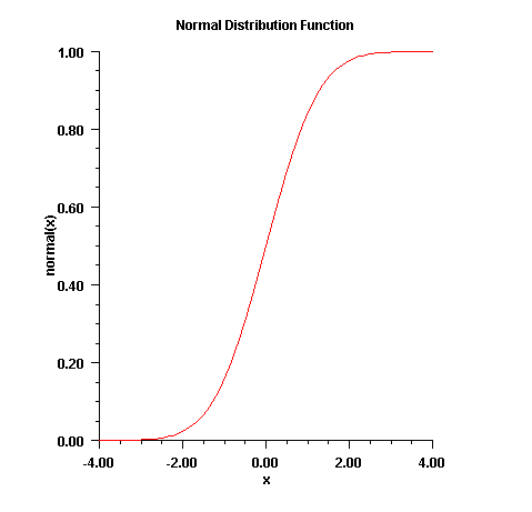
See Also:: Example

normal

public static double normal(double x)

Evaluates the normal (Gaussian) cumulative probability distribution function.

Method normal evaluates the distribution function, , of a standard normal (Gaussian) random variable, that is,

$Phi left( x right) = frac{1}{{sqrt {2pi } }}int_{ - infty }^x {} e^{ - t^2 /2} dt$

The value of the distribution function at the point x is the probability that the random variable takes a value less than or equal to x.

The standard normal distribution (for which normal is the distribution function) has mean of 0 and variance of 1. The probability that a normal random variable with mean and variance is less than y is given by normal evaluated at .

is evaluated by use of the complementary error function, erfc. The relationship is:

Standard Normal Distribution Function

Parameters:: x - a double scalar value representing the argument at which the function is to be evaluated.
Returns:: a double scalar value representing the probability that a normal variable takes a value less than or equal to x.
See Also:: Example

Pareto

public static double Pareto(double x,
                            double xm,
                            double k)

Evaluates the Pareto cumulative probability distribution function.

Method Pareto evaluates the distribution function, F, of a Pareto random variable with scale parameter and shape parameter k. It is given by

$F(x,x_m,k)=1-left ( frac{x_m}{x} right )^{k}$

where and . The function is only defined for

Parameters:: x - a double scalar value representing the argument at which the function is to be evaluated.; xm - a double scalar value representing the scale parameter, .; k - a double scalar value representing the shape parameter, .
Returns:: a double scalar value representing the probability that a Pareto random variable takes a value less than or equal to x.

poisson

public static double poisson(int k,
                             double theta)

Evaluates the Poisson cumulative probability distribution function.

poisson evaluates the distribution function of a Poisson random variable with parameter theta. theta, which is the mean of the Poisson random variable, must be positive. The probability function (with ) is

$f(x) = e^{ - theta } theta ^x /x!,,, for,x = 0,,1,,2,, ldots$

The individual terms are calculated from the tails of the distribution to the mode of the distribution and summed. poisson uses the recursive relationship

with $f(0) = e^{-theta}$ .

Parameters:: k - the int argument for which the Poisson distribution function is to be evaluated.; theta - a double scalar value representing the mean of the Poisson distribution.
Returns:: a double scalar value representing the probability that a Poisson random variable takes a value less than or equal to k.
See Also:: Example

Rayleigh

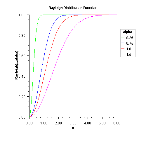
public static double Rayleigh(double x,
                              double alpha)

Evaluates the Rayleigh cumulative probability distribution function.

Method Rayleigh is a special case of Weibull distribution function where the shape parameter gamma is 2.0; that is,

$F(x) = 1-e^{-frac{x^2}{2alpha^2}}$

where alpha is the scale parameter.

Plot of Rayleigh Distribution Function

Parameters:: x - a double scalar value representing the argument at which the function is to be evaluated. It must be non-negative.; alpha - a double scalar value representing the scale parameter.
Returns:: a double scalar value representing the probability that a Rayleigh random variable takes a value less than or equal to x.

studentsT

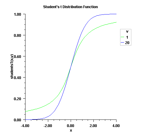
public static double studentsT(double t,
                               double df)

Evaluates the Student's t cumulative probability distribution function.

Method studentsT evaluates the distribution function of a Student's t random variable with df degrees of freedom. If the square of t is greater than or equal to df, the relationship of a t to an f random variable (and subsequently, to a beta random variable) is exploited, and routine beta is used. Otherwise, the method described by Hill (1970) is used. If df is not an integer, if df is greater than 19, or if df is greater than 200, a Cornish-Fisher expansion is used to evaluate the distribution function. If df is less than 20 and is less than 2.0, a trigonometric series (see Abramowitz and Stegun 1964, equations 26.7.3 and 26.7.4, with some rearrangement) is used. For the remaining cases, a series given by Hill (1970) that converges well for large values of t is used.

For greater right tail accuracy, see complementaryStudentsT(double, double).

Student's t Distribution Function

Parameters:: t - a double scalar value representing the argument at which the function is to be evaluated; df - a double scalar value representing the number of degrees of freedom. This must be at least one.
Returns:: a double scalar value representing the probability that a Student's t random variable takes a value less than or equal to t.
See Also:: Example

uniform

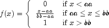
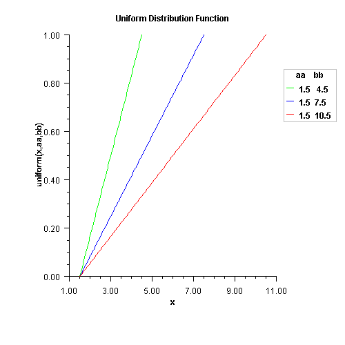
public static double uniform(double x,
                             double aa,
                             double bb)

Evaluates the uniform cumulative probability distribution function.

Method uniform evaluates the distribution function, F, of a uniform random variable with location parameter aa and scale parameter bb; that is,

$f(x)=left{begin{array}{cl} 0 & mbox{if}~ x lt aa \ frac{x-aa}{bb-aa} & mbox{if}~ aale xle bb \ 1 &mbox{if}~ x>bb end{array}right.$

Plot of Uniform Distribution Function

Parameters:: x - a double scalar value representing the argument at which the function is to be evaluated.; aa - a double scalar value representing the location parameter.; bb - a double scalar value representing the scale parameter.
Returns:: a double scalar value representing the probability that a uniform random variable takes a value less than or equal to x.

Weibull

public static double Weibull(double x,
                             double gamma,
                             double alpha)

Evaluates the Weibull cumulative probability distribution function.

Method Weibull evaluates the distribution function given by

$F(x,gamma,alpha)=1-e^{-(x/alpha)^{gamma}}$

Parameters:: x - a double scalar value representing the argument at which the function is to be evaluated. It must be non-negative.; gamma - a double scalar value representing the shape parameter, .; alpha - a double scalar value representing the scale parameter, .
Returns:: a double scalar value representing the probability that a Weibull random variable takes a value less than or equal to x.