Class Cdf
-
Method Summary
Modifier and TypeMethodDescriptionstatic doublebeta(double x, double pin, double qin) Evaluates the beta cumulative probability distribution function.static doublebetaMean(double pin, double qin) Evaluates the mean of the beta cumulative probability distribution functionstatic doublebetaProb(double x, double pin, double qin) Deprecated.static doublebetaVariance(double pin, double qin) Evaluates the variance of the beta cumulative probability distribution functionstatic doublebinomial(int k, int n, double pin) Evaluates the binomial cumulative probability distribution function.static doublebinomialProb(int k, int n, double pin) Deprecated.UsePdf.binomial(int, int, double)instead.static doublebivariateNormal(double x, double y, double rho) Evaluates the bivariate normal cumulative probability distribution function.static doublechi(double chsq, double df) Evaluates the chi-squared cumulative distribution function.static doublechiMean(double df) Evaluates the mean of the chi-squared cumulative probability distribution functionstatic doublechiProb(double chsq, double df) Deprecated.UsePdf.chi(double, double)instead.static doublechiVariance(double df) Evaluates the variance of the chi-squared cumulative probability distribution functionstatic doublecomplementaryChi(double chsq, double df) Calculates the complement of the chi-squared cumulative distribution function.static doublecomplementaryF(double x, double dfn, double dfd) Calculates the complement of the F distribution function.static doublecomplementaryF2(double x, double dfn, double dfd) static doublecomplementaryNoncentralF(double f, double df1, double df2, double lambda) Calculates the complement of the noncentral F cumulative distribution function.static doublecomplementaryStudentsT(double t, double df) Calculates the complement of the Student's t distribution.static doublecontinuousUniform(double x, double a, double b) Evaluates the continuous uniform cumulative distribution function.static doublediscreteUniform(int x, int n) Evaluates the discrete uniform cumulative probability distribution function.static doublediscreteUniformProb(int x, int n) Deprecated.UsePdf.discreteUniform(int, int)instead.static doubleexponential(double x, double scale) Evaluates the exponential cumulative probability distribution function.static doubleexponentialProb(double x, double scale) Deprecated.UsePdf.exponential(double, double)instead.static doubleextremeValue(double x, double mu, double beta) Evaluates the extreme value cumulative probability distribution function.static doubleextremeValueProb(double x, double mu, double beta) Deprecated.UsePdf.extremeValue(double, double, double)instead.static doubleF(double x, double dfn, double dfd) Evaluates the F cumulative probability distribution function.static doubleFProb(double x, double dfn, double dfd) Deprecated.UsePdf.F(double, double, double)instead.static doublegamma(double x, double a) Evaluates the gamma cumulative probability distribution function.static doublegammaProb(double x, double a, double b) Deprecated.UsePdf.gamma(double, double, double)instead.static doublegeneralizedExtremeValue(double x, double mu, double sigma, double xi) Evaluates the generalized extreme value cumulative distribution function.static doublegeneralizedGaussian(double x, double mu, double alpha, double beta) Evaluates the generalized Gaussian (normal) cumulative distribution function.static doublegeneralizedPareto(double x, double mu, double sigma, double alpha) Evaluates the generalized Pareto cumulative distribution function.static doublegeometric(int x, double pin) Evaluates the discrete geometric cumulative probability distribution function.static doublegeometricProb(int x, double pin) Deprecated.UsePdf.geometric(int, double)instead.static doublehypergeometric(int k, int sampleSize, int defectivesInLot, int lotSize) Evaluates the hypergeometric cumulative probability distribution function.static doublehypergeometricProb(int k, int sampleSize, int defectivesInLot, int lotSize) Deprecated.UsePdf.hypergeometric(int, int, int, int)instead.static doubleinverseBeta(double p, double pin, double qin) Deprecated.UseInvCdf.beta(double, double, double)instead.static doubleinverseChi(double p, double df) Deprecated.UseInvCdf.chi(double, double)instead.static intinverseDiscreteUniform(double p, int n) Deprecated.UseInvCdf.discreteUniform(double, int)instead.static doubleinverseExponential(double p, double scale) Deprecated.UseInvCdf.exponential(double, double)instead.static doubleinverseExtremeValue(double p, double mu, double beta) Deprecated.UseInvCdf.extremeValue(double, double, double)instead.static doubleinverseF(double p, double dfn, double dfd) Deprecated.UseInvCdf.F(double, double, double)instead.static doubleinverseGamma(double p, double a) Deprecated.UseInvCdf.gamma(double, double)instead.static doubleinverseGeometric(double r, double pin) Deprecated.UseInvCdf.geometric(double, double)instead.static doubleinverseLogNormal(double p, double mu, double sigma) Deprecated.UseInvCdf.logNormal(double, double, double)instead.static doubleinverseNoncentralchi(double p, double df, double alam) Deprecated.UseInvCdf.noncentralchi(double, double, double)instead.static doubleinverseNoncentralstudentsT(double p, int idf, double delta) Deprecated.UseInvCdf.noncentralstudentsT(double, int, double)instead.static doubleinverseNormal(double p) Deprecated.UseInvCdf.normal(double)instead.static doubleinverseRayleigh(double p, double alpha) Deprecated.UseInvCdf.Rayleigh(double, double)instead.static doubleinverseStudentsT(double p, double df) Deprecated.UseInvCdf.studentsT(double, double)instead.static doubleinverseUniform(double p, double aa, double bb) Deprecated.UseInvCdf.uniform(double, double, double)instead.static doubleinverseWeibull(double p, double gamma, double alpha) Deprecated.UseInvCdf.Weibull(double, double, double)instead.static doublelogistic(double x, double mu, double sigma) Evaluates the logistic cumulative probability distribution function.static doublelogNormal(double x, double mu, double sigma) Evaluates the standard lognormal cumulative probability distribution function.static doublelogNormalProb(double x, double mu, double sigma) Deprecated.UsePdf.logNormal(double, double, double)instead.static doublenoncentralBeta(double x, double shape1, double shape2, double lambda) Evaluates the noncentral beta cumulative distribution function (CDF).static doublenoncentralchi(double chsq, double df, double alam) Evaluates the noncentral chi-squared cumulative probability distribution function.static doublenoncentralF(double f, double df1, double df2, double lambda) Evaluates the noncentral F cumulative distribution function.static doublenoncentralstudentsT(double t, int idf, double delta) Evaluates the noncentral Student's t cumulative probability distribution function.static doublenormal(double x) Evaluates the standard normal (Gaussian) cumulative probability distribution function.static doublePareto(double x, double xm, double k) Evaluates the Pareto cumulative probability distribution function.static doublepoisson(int k, double theta) Evaluates the Poisson cumulative probability distribution function.static doublepoissonProb(int k, double theta) Deprecated.UsePdf.poisson(int, double)instead.static doubleRayleigh(double x, double alpha) Evaluates the Rayleigh cumulative probability distribution function.static doubleRayleighProb(double x, double alpha) Deprecated.UsePdf.Rayleigh(double, double)instead.static doublestudentsT(double t, double df) Evaluates the Student's t cumulative probability distribution function.static doubleuniform(double x, double aa, double bb) Deprecated.usecontinuousUniform(double, double, double)insteadstatic doubleWeibull(double x, double gamma, double alpha) Evaluates the Weibull cumulative probability distribution function.static doubleWeibullProb(double x, double gamma, double alpha) Deprecated.UsePdf.Weibull(double, double, double)instead.
-
Method Details
-
binomial
public static double binomial(int k, int n, double pin) Evaluates the binomial cumulative probability distribution function.Method
binomialevaluates the distribution function of a binomial random variable with parameters n and p with p=pin. It does this by summing probabilities of the random variable taking on the specific values in its range. These probabilities are computed by the recursive relationship$$\Pr \left( {X = j} \right) = \frac{{\left( {n + 1 - j} \right)p}}{{j\left( {1 - p} \right)}}\Pr \left( {X = j - 1} \right)$$
To avoid the possibility of underflow, the probabilities are computed forward from 0, if k is not greater than n times p, and are computed backward from n, otherwise. The smallest positive machine number, \(\varepsilon\), is used as the starting value for summing the probabilities, which are rescaled by \((1 - p)^n\varepsilon\) if forward computation is performed and by \(p^n\varepsilon\) if backward computation is done. For the special case of p = 0,
binomialis set to 1; and for the case p = 1,binomialis set to 1 if k = n and to 0 otherwise.- Parameters:
k- theintargument for which the binomial distribution function is to be evaluated.n- theintnumber of Bernoulli trials.pin- adouble, the probability of success on each independent trial.- Returns:
- a
double, the probability that a binomial random variable takes a value less than or equal tok. This value is the probability thatkor fewer successes occur innindependent Bernoulli trials, each of which has apinprobability of success. - See Also:
-
bivariateNormal
public static double bivariateNormal(double x, double y, double rho) Evaluates the bivariate normal cumulative probability distribution function. Let \((X,Y)\) be a bivariate normal variable with mean \((0,0)\) and variance-covariance matrix $$ \left[ \begin{array}{cc} 1 & \rho \\ \rho & 1\end{array}\right] $$ This method computes the probability that \(X \le {\tt x}\) and \(Y \le {\tt y}\).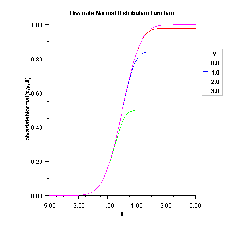
- Parameters:
x- is the x-coordinate of the point for which the bivariate normal distribution function is to be evaluated.y- is the y-coordinate of the point for which the bivariate normal distribution function is to be evaluated.rho- is the correlation coefficient.- Returns:
- the probability that a bivariate normal random variable
\((X,Y)\)
with correlation
rhosatisfies \(X \le {\tt x}\) and \(Y \le {\tt y}\).
-
poisson
public static double poisson(int k, double theta) Evaluates the Poisson cumulative probability distribution function.poissonevaluates the distribution function of a Poisson random variable with parametertheta.theta, which is the mean of the Poisson random variable, must be positive. The probability function (with \(\theta = theta\)) is$$f(x) = e^{ - \theta } \theta ^x /x!\,\,\, for\,x = 0,\,1,\,2,\, \ldots $$
The individual terms are calculated from the tails of the distribution to the mode of the distribution and summed.
poissonuses the recursive relationship$$f\left( {x + 1} \right) = f\left( x \right) (\theta /\left( {x + 1} \right)),\,\,\,for\,x = 0,\,1,\,2,\, \ldots k-1$$
with \(f(0) = e^{-\theta}\).
- Parameters:
k- theintargument for which the Poisson distribution function is to be evaluatedtheta- adouble, the mean of the Poisson distribution- Returns:
- a
double, the probability that a Poisson random variable takes a value less than or equal to k - See Also:
-
betaMean
public static double betaMean(double pin, double qin) Evaluates the mean of the beta cumulative probability distribution function- Parameters:
pin- adouble, the first beta distribution parameter.qin- adouble, the second beta distribution parameter.- Returns:
- a
double, the mean of the beta distribution function.
-
betaVariance
public static double betaVariance(double pin, double qin) Evaluates the variance of the beta cumulative probability distribution function- Parameters:
pin- adouble, the first beta distribution parameter.qin- adouble, the second beta distribution parameter.- Returns:
- a
double, the variance of the beta distribution function.
-
F
public static double F(double x, double dfn, double dfd) Evaluates the F cumulative probability distribution function.Fevaluates the distribution function of a Snedecor's F random variable withdfnnumerator degrees of freedom anddfddenominator degrees of freedom. The function is evaluated by making a transformation to a beta random variable and then using the functionbeta. If X is an F variate with \(v_1\) and \(v_2\) degrees of freedom and \(Y = v_1X/(v_2 + v_1X)\), then Y is a beta variate with parameters \(p = v_1/2\) and \(q = v_2/2\).Falso uses a relationship between F random variables that can be expressed as follows:$${\rm F}(X, {\it dfn}, {\it dfd})= {\rm F}(1/X, {\it dfd}, {\it dfn})$$
For greater right tail accuracy, see
complementaryF(double, double, double).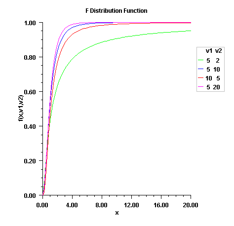
- Parameters:
x- adouble, the argument at which the function is to be evaluated.dfn- adouble, the numerator degrees of freedom. It must be positive.dfd- adouble, the denominator degrees of freedom. It must be positive.- Returns:
- a
double, the probability that an F random variable takes on a value less than or equal tox. - See Also:
-
complementaryF
public static double complementaryF(double x, double dfn, double dfd) Calculates the complement of the F distribution function.complementaryFevaluates one minus the distribution function of a Snedecor's F random variable withdfnnumerator degrees of freedom anddfddenominator degrees of freedom. The function is evaluated by making a transformation to a beta random variable and then using the functionbeta. If X is an F variate with \(v_1\) and \(v_2\) degrees of freedom and \(Y = v_1X/(v_2 + v_1X)\), then Y is a beta variate with parameters \(p = v_1/2\) and \(q = v_2/2\).complementaryFalso uses a relationship between F random variables that can be expressed as follows:$${\rm F}(X, {\it dfn}, {\it dfd})= {\rm F}(1/X, {\it dfd}, {\it dfn})$$
This function provides higher right tail accuracy for the F distribution.
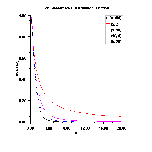
- Parameters:
x- adouble, the argument at which \( Pr\left( x \gt F \right)\) is to be evaluated.dfn- adouble, the numerator degrees of freedom. It must be positive.dfd- adouble, the denominator degrees of freedom. It must be positive.- Returns:
- a
double, the probability that an F random variable takes on a value greater thanx.
-
complementaryF2
public static double complementaryF2(double x, double dfn, double dfd) -
hypergeometric
public static double hypergeometric(int k, int sampleSize, int defectivesInLot, int lotSize) Evaluates the hypergeometric cumulative probability distribution function.Method
hypergeometricevaluates the distribution function of a hypergeometric random variable with parameters n, l, and m. The hypergeometric random variable X can be thought of as the number of items of a given type in a random sample of size n that is drawn without replacement from a population of size l containing m items of this type. The probability function is$$\Pr \left( {X = j} \right) = \frac{{\left( {_j^m } \right)\left( {_{n - j}^{l - m} } \right)}}{{\left( {_n^l } \right)}}{\rm{for }}\,\,j = i,\;i + 1,\,\,i + 2,\; \ldots ,\;\min \left( {n,m} \right)$$
where \(i = {\rm max}(0, n - l + m)\).
If k is greater than or equal to i and less than or equal to \(\min (n, m)\),
hypergeometricsums the terms in this expression for j going from i up to k. Otherwise,hypergeometricreturns 0 or 1, as appropriate. So, as to avoid rounding in the accumulation,hypergeometricperforms the summation differently depending on whether or not k is greater than the mode of the distribution, which is the greatest integer less than or equal to \((m + 1)(n + 1)/(l + 2)\).- Parameters:
k- anint, the argument at which the function is to be evaluated.sampleSize- anint, the sample size,n.defectivesInLot- anint, the number of defectives in the lot,m.lotSize- anint, the lot size,l.- Returns:
- a
double, the probability that a hypergeometric random variable takes a value less than or equal tok. - See Also:
-
gamma
public static double gamma(double x, double a) Evaluates the gamma cumulative probability distribution function.Method
gammaevaluates the distribution function, F, of a gamma random variable with shape parameter a; that is,$$F\left( x \right) = \frac{1}{{\Gamma \left( a \right)}}\int_0^x {e^{ - t} t^{a - 1} } dt $$
where \(\Gamma(\cdot)\) is the gamma function. (The gamma function is the integral from 0 to \(\infty\) of the same integrand as above). The value of the distribution function at the point x is the probability that the random variable takes a value less than or equal to x.
The gamma distribution is often defined as a two-parameter distribution with a scale parameter b (which must be positive), or even as a three-parameter distribution in which the third parameter c is a location parameter. In the most general case, the probability density function over \((c, \infty)\) is
$$f\left( t \right) = \frac{1}{{b^a \Gamma \left( a \right)}}e^{ - \left( {t - c} \right)/b} \left( {x - c} \right)^{a - 1}$$
If T is such a random variable with parameters a, b, and c, the probability that \(T \le t_0\) can be obtained from
gammaby setting \(X = (t_0 - c)/b\).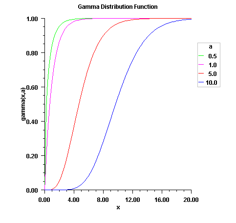
- Parameters:
x- adouble, the argument at which the function is to be evaluateda- adouble, the shape parameter. This must be positive.- Returns:
- a
double,the probability that a gamma random variable takes on a value less than or equal tox - See Also:
-
exponential
public static double exponential(double x, double scale) Evaluates the exponential cumulative probability distribution function.Method
exponentialis a special case of the gamma distribution function, which evaluates the distribution function, F, with scale parameter b and shape parameter a, used in the gamma distribution function equal to 1.0. That is,$$F\left( x \right) = \frac{1}{{\Gamma \left( a \right)}}\int_0^x {e^{ - t/b}} dt$$
where \(\Gamma(\cdot)\) is the gamma function. (The gamma function is the integral from 0 to \(\infty\) of the same integrand as above). The value of the distribution function at the point x is the probability that the random variable takes a value less than or equal to x.
If
xis less than or equal to 1.0,gammauses a series expansion. Otherwise, a continued fraction expansion is used. (See Abramowitz and Stegun, 1964.)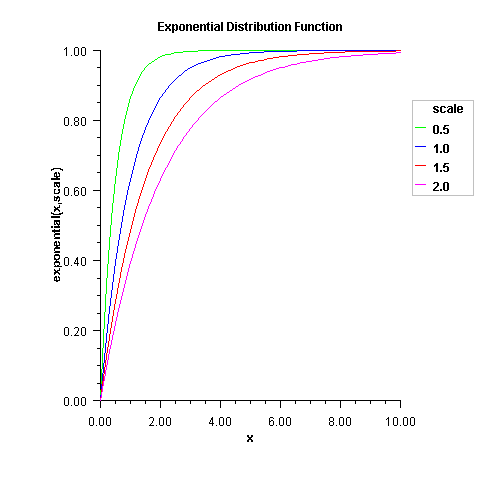
- Parameters:
x- adoublethe argument at which the function is to be evaluatedscale- adouble, the scale parameter, \(b\)- Returns:
- a
double, the probability that an exponential random variable takes on a value less than or equal tox - See Also:
-
normal
public static double normal(double x) Evaluates the standard normal (Gaussian) cumulative probability distribution function.Method
normalevaluates the distribution function, \(\Phi\), of a standard normal (Gaussian) random variable, that is,$$\Phi \left( x \right) = \frac{1}{{\sqrt {2\pi } }}\int_{ - \infty }^x {} e^{ - t^2 /2} dt$$
The value of the distribution function at the point x is the probability that the random variable takes a value less than or equal to x.
The standard normal distribution (for which
normalis the distribution function) has mean of 0 and variance of 1. The probability that a normal random variable with mean \(\mu\) and variance \(\sigma^2\) is less than y is given bynormalevaluated at \((y - \mu)/\sigma\).\(\Phi(x)\) is evaluated by use of the complementary error function, erfc. The relationship is:
$$\Phi (x) = {\rm{erfc}}( - x/ \sqrt {2.0}) /2$$
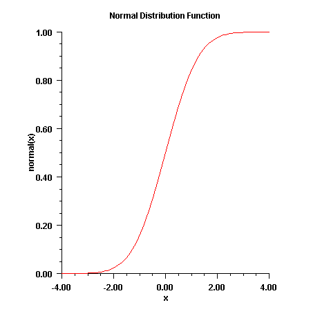
- Parameters:
x- adouble, the argument at which the function is to be evaluated- Returns:
- a
double, the probability that a normal variable takes a value less than or equal tox - See Also:
-
chiMean
public static double chiMean(double df) Evaluates the mean of the chi-squared cumulative probability distribution function- Parameters:
df- adouble, the number of degrees of freedom. This must be at least 0.5.- Returns:
- a
double, the mean of the chi-squared distribution function
-
chiVariance
public static double chiVariance(double df) Evaluates the variance of the chi-squared cumulative probability distribution function- Parameters:
df- adouble, the number of degrees of freedom. This must be at least 0.5.- Returns:
- a
double, the variance of the chi-squared distribution function
-
chi
public static double chi(double chsq, double df) Evaluates the chi-squared cumulative distribution function.Method
chievaluates the cumulative distribution function (CDF) F, of a chi-squared random variable withdfdegrees of freedom, that is, with x =chsqand \(\nu\) =df,$$F\left( x, \nu \right) \;=\; \frac{1}{{2^{\nu /2} \Gamma \left( {\nu /2} \right)}} \int_0^x {e^{ - t/2} t^{\nu /2 - 1} } dt$$
where \(\Gamma (\cdot)\) is the gamma function. The value \(p \;=\; F\left( x, \nu \right)\) is the probability that the random variable takes a value less than or equal to x.
For \(\nu \;>\; 343\),
chiuses the Wilson-Hilferty approximation (Abramowitz and Stegun [A&S] 1964, equation 26.4.17) for p in terms of the normal CDF, which is evaluated using methodnormal.For \(\nu \;\le\; 343\),
chiuses series expansions to evaluate p: for \(x \;\lt\; \nu\),chicalculates p using A&S equation 6.5.29, and for \(x \;\ge\; \nu\),chicalculates p using the continued fraction (CF) expansion of the incomplete gamma function given in A&S equation 6.5.31 and implemented using Lentz's algorithm (Lentz, W.J., 1976, Applied Optics, vol. 15, pp. 668-671) as modified by Thompson & Barnett (Thompson, I.J., and Barnett, A.R., 1986, Journal of Computational Physics, vol. 64, pp. 490-509).For greater right tail accuracy, see
complementaryChi(double, double).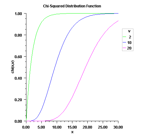
- Parameters:
chsq- adouble, the argument at which the function is to be evaluateddf- adouble, the number of degrees of freedom.dfmust be positive.- Returns:
- a
double, the probability that a chi-squared random variable takes a value less than or equal tochsq - See Also:
-
complementaryChi
public static double complementaryChi(double chsq, double df) Calculates the complement of the chi-squared cumulative distribution function.Method
complementaryChievaluates the cumulative distribution function, \(1-F\), of a chi-squared random variable withdfdegrees of freedom, that is, with x =chsqand \(\nu\) =df,$$p \;=\; F\left( x, \nu \right) \;=\; \frac{1}{{2^{\nu /2} \Gamma \left( {\nu /2} \right)}} \int_0^x {e^{ - t/2} t^{\nu /2 - 1} } dt$$
where \(\Gamma (\cdot)\) is the gamma function. The value of the
complementaryChidistribution function at the point x, \(1 - p\), is the probability that the random variable takes a value greater than x.For \(\nu \;>\; 343\),
complementaryChiuses the Wilson-Hilferty approximation (Abramowitz and Stegun [A&S] 1964, equation 26.4.17) for p in terms of the normal CDF, which is evaluated using methodnormal.For \(\nu \;\le\; 343\),
complementaryChiuses series expansions to evaluate p: for \(x \;\lt\; \nu\),complementaryChicalculates p using A&S series 6.5.29, and for \(x \;\ge\; \nu\),complementaryChicalculates p using the continued fraction expansion of the incomplete gamma function given in A&S equation 6.5.31 and implemented using Lentz's algorithm (Lentz, W.J., 1976, Applied Optics, vol. 15, pp. 668-671) as modified by Thompson & Barnett (Thompson, I.J., and Barnett, A.R., 1986, Journal of Computational Physics, vol. 64, pp. 490-509).complementaryChiprovides greater right tail accuracy for the Chi-squared distribution than does1 - chi.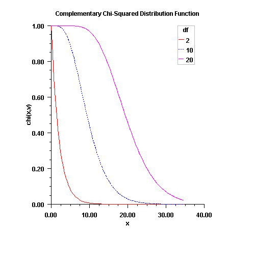
- Parameters:
chsq- adouble, the value at which the function is to be evaluateddf- adouble, the number of degrees of freedom.dfmust be positive.- Returns:
- a
double, the probability that a chi-squared random variable takes a value greater thanchsq
-
noncentralBeta
public static double noncentralBeta(double x, double shape1, double shape2, double lambda) Evaluates the noncentral beta cumulative distribution function (CDF).The noncentral beta distribution is a generalization of the beta distribution. If \(Z\) is a noncentral chi-square random variable with noncentrality parameter \(\lambda\) and \(2 \alpha_1\) degrees of freedom, and \(Y\) is a chi-square random variable with \(2 \alpha_2\) degrees of freedom which is statistically independent of \(Z\), then
$$X \;\; = \;\; \frac{Z}{Z \; + \; Y} \;\; = \;\; \frac{\alpha_1 F}{\alpha_1 F \; + \; \alpha_2}$$
is a noncentral beta-distributed random variable and
$$F \;\; = \;\; \frac{\alpha_2 Z}{\alpha_1 Y} \;\; = \;\; \frac{\alpha_2 X}{\alpha_1 (1 \; - \; X)}$$
is a noncentral F-distributed random variable. The CDF for noncentral beta variable X can thus be simply defined in terms of the noncentral F CDF:
$$CDF_{nc\beta}(x, \; \alpha_1, \; \alpha_2, \; \lambda) \;\; = \;\; CDF_{ncF}(f, \; 2 \alpha_1, \; 2 \alpha_2, \; \lambda)$$
where \(CDF_{nc\beta}(x, \; \alpha_1, \; \alpha_2, \; \lambda)\) is the noncentral beta CDF with \(x\) =
x, \(\alpha_1\) =shape1, \(\alpha_2\) =shape2, and noncentrality parameter \(\lambda\) =lambda; \(CDF_{ncF}(f, \; 2 \alpha_1, \; 2 \alpha_2, \; \lambda)\) is the noncentral F CDF with argument f, numerator and denominator degrees of freedom \(2 \alpha_1\) and \(2 \alpha_2\) respectively, and noncentrality parameter \(\lambda\); and:$$f \;\; = \;\; \frac{\alpha_2 x}{\alpha_1 (1 \; - \; x)}; \;\; x \;\; = \;\; \frac{\alpha_1 f}{\alpha_1 f \; + \; \alpha_2}$$
(See documentation for class
CdfmethodnoncentralFfor a discussion of how the noncentral F CDF is defined and calculated.)With a noncentrality parameter of zero, the noncentral beta distribution is the same as the beta distribution.
- Parameters:
x- adouble, the argument at which the function is to be evaluatedxmust be nonnegative and less than or equal to 1.shape1- adouble, the first shape parameter.shape1must be positive.shape2- adouble, the second shape parameter.shape2must be positive.lambda- adouble, the noncentrality parameter.lambdamust nonnegative.- Returns:
- a
double, the probability that a noncentral beta random variable takes a value less than or equal tox
-
noncentralchi
public static double noncentralchi(double chsq, double df, double alam) Evaluates the noncentral chi-squared cumulative probability distribution function.Method
noncentralchievaluates the distribution function, F, of a noncentral chi-squared random variable withdfdegrees of freedom and noncentrality parameteralam, that is, with \(\nu = {\rm df}\), \(\lambda = {\rm alam}\), and \(\chi = {\rm chsq}\),$$F\left( x \right) = \sum\limits_{i = 0}^\infty {\frac{e^{-\lambda/2}\left(\lambda/2\right)^i}{i!}} \int_0^x {\frac{t^{\left(\nu + 2i\right)/2-1}e^{ - t/2}} {2^{\left(\nu+2i\right)/2}{\Gamma\left(\frac{\nu+2i}{2}\right)}}} dt$$
where \(\Gamma (\cdot)\) is the gamma function. This is a series of central chi-squared distribution functions with Poisson weights. The value of the distribution function at the point x is the probability that the random variable takes a value less than or equal to x.
The noncentral chi-squared random variable can be defined by the distribution function above, or alternatively and equivalently, as the sum of squares of independent normal random variables. If the \(Y_i\) have independent normal distributions with means \({\mu}_i\) and variances equal to one and
$$X = \sum\limits_{i = 1}^n{Y_i}^2 $$
then \(X\) has a noncentral chi-squared distribution with \(n\) degrees of freedom and noncentrality parameter equal to
$$\sum\limits_{i = 1}^n{\mu_i}^2$$
With a noncentrality parameter of zero, the noncentral chi-squared distribution is the same as the chi-squared distribution.
noncentralchidetermines the point at which the Poisson weight is greatest, and then sums forward and backward from that point, terminating when the additional terms are sufficiently small or when a maximum of 1000 terms have been accumulated. The recurrence relation 26.4.8 of Abramowitz and Stegun (1964) is used to speed the evaluation of the central chi-squared distribution functions.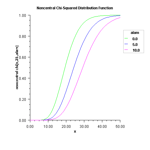
- Parameters:
chsq- adouble, the argument at which the function is to be evaluateddf- adouble, the number of degrees of freedom.dfmust be positive.alam- adouble, the noncentrality parameter. This must be nonnegative, andalam + dfmust be less than or equal to 200,000.- Returns:
- a
double, the probability that a chi-squared random variable takes a value less than or equal tochsq - See Also:
-
studentsT
public static double studentsT(double t, double df) Evaluates the Student's t cumulative probability distribution function.Method
studentsTevaluates the distribution function of a Student's t random variable withdfdegrees of freedom. If the square of t is greater than or equal todf, the relationship of a t to an f random variable (and subsequently, to a beta random variable) is exploited, and routinebetais used. Otherwise, the method described by Hill (1970) is used. Ifdfis not an integer, ifdfis greater than 19, or ifdfis greater than 200, a Cornish-Fisher expansion is used to evaluate the distribution function. Ifdfis less than 20 and \(\left|{\rm t}\right|\) is less than 2.0, a trigonometric series (see Abramowitz and Stegun 1964, equations 26.7.3 and 26.7.4, with some rearrangement) is used. For the remaining cases, a series given by Hill (1970) that converges well for large values oftis used.For greater right tail accuracy, see
complementaryStudentsT(double, double).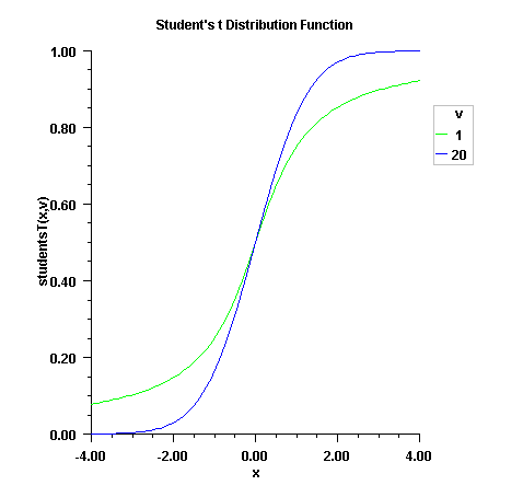
- Parameters:
t- adouble, the argument at which the function is to be evaluateddf- adouble, the number of degrees of freedom. This must be at least one.- Returns:
- a
double, the probability that a Student's t random variable takes a value less than or equal tot - See Also:
-
complementaryStudentsT
public static double complementaryStudentsT(double t, double df) Calculates the complement of the Student's t distribution.Method
complementaryStudentsTevaluates one minus the distribution function of a Student's t random variable withdfdegrees of freedom. If the square of t is greater than or equal todf, the relationship of a t to an f random variable (and subsequently, to a beta random variable) is exploited, and routinebetais used. Otherwise, the method described by Hill (1970) is used. Ifdfis not an integer, ifdfis greater than 19, or ifdfis greater than 200, a Cornish-Fisher expansion is used to evaluate the distribution function. Ifdfis less than 20 and \(\left|{\rm t}\right|\) is less than 2.0, a trigonometric series (see Abramowitz and Stegun 1964, equations 26.7.3 and 26.7.4, with some rearrangement) is used. For the remaining cases, a series given by Hill (1970) that converges well for large values oftis used.This function provides higher right tail accuracy for the Student's t distribution.
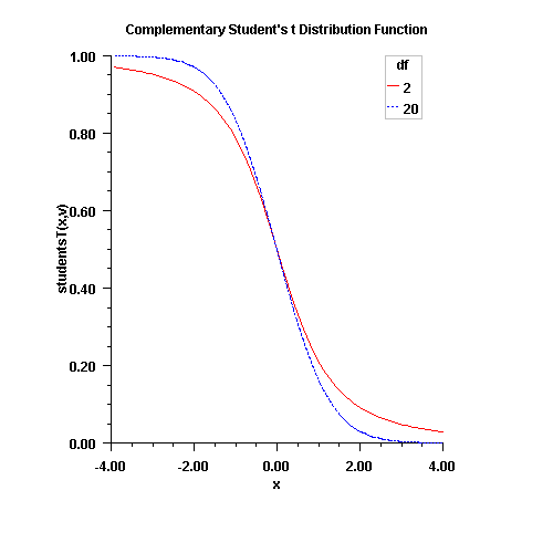
- Parameters:
t- adoublescalar value for which \( Pr\left( x \gt t \right)\)is to be evaluateddf- adouble, the number of degrees of freedom. This must be at least one.- Returns:
- a
double, the probability that a Student's t random variable takes a value greater thant - See Also:
-
noncentralstudentsT
public static double noncentralstudentsT(double t, int idf, double delta) Evaluates the noncentral Student's t cumulative probability distribution function.Method
noncentralstudentsTevaluates the distribution functionFof a noncentral t random variable withidfdegrees of freedom and noncentrality parameterdelta; that is, with \(\nu = idf\), \(\delta = delta\), and \(t_{0}= t\),$$F{\left({t_0}\right)} = \int_{-{\infty}}^{t_{0}} {\frac {\nu^{\nu/2}e^{{-\delta^2}/2}} {{\sqrt{\pi}\Gamma\left(\nu/2\right)\left(\nu+x^2\right)}^{\left(\nu+1\right)/2}} } \sum\limits_{i = 0}^\infty {\Gamma\left(\left(\nu+i+1\right)/2\right)\left(\frac{\delta^i}{i!}\right)\left(\frac{2x^2}{\nu+x^2}\right)^{i/2} dx }$$
where \(\Gamma (\cdot)\) is the gamma function. The value of the distribution function at the point \(t_{0}\) is the probability that the random variable takes a value less than or equal to \(t_{0}\).
The noncentral t random variable can be defined by the distribution function above, or alternatively and equivalently, as the ratio of a normal random variable and an independent chi-squared random variable. If w has a normal distribution with mean \(\delta\) and variance equal to one, \(u\) has an independent chi-squared distribution with \(\nu\) degrees of freedom, and
$$x = w/\sqrt{u/\nu}$$
then \(x\) has a noncentral \(t\) distribution with \(\nu\) degrees of freedom and noncentrality parameter \(\delta\).
The distribution function of the noncentral \(t\) can also be expressed as a double integral involving a normal density function (see, for example, Owen 1962, page 108). The method
noncentralstudentsTuses the method of Owen (1962, 1965), which uses repeated integration by parts on that alternate expression for the distribution function.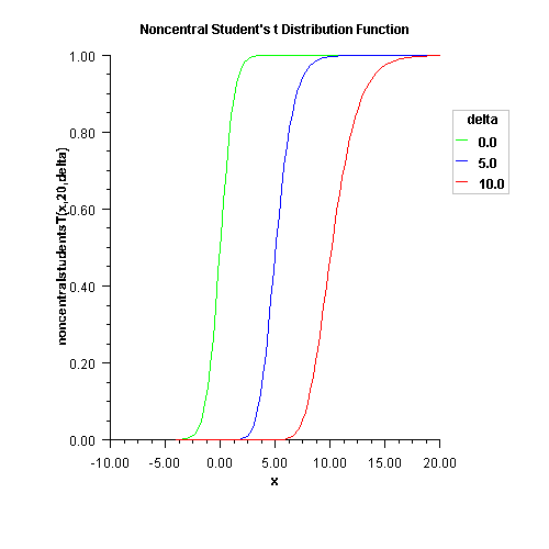
- Parameters:
t- adouble, the argument at which the function is to be evaluatedidf- anint, the number of degrees of freedom. This must be positive.delta- adouble, the noncentrality parameter- Returns:
- a
double, the probability that a noncentral Student's t random variable takes a value less than or equal tot - See Also:
-
Weibull
public static double Weibull(double x, double gamma, double alpha) Evaluates the Weibull cumulative probability distribution function.Method
Weibullevaluates the distribution function given by$$F(x,\gamma,\alpha)=1-e^{-(x/\alpha)^{\gamma}}$$
- Parameters:
x- adouble, the argument at which the function is to be evaluated. It must be non-negative.gamma- adouble, the shape parameter, \(\gamma\)alpha- adouble, the scale parameter, \(\alpha\)- Returns:
- a
double, the probability that a Weibull random variable takes a value less than or equal tox
-
logNormal
public static double logNormal(double x, double mu, double sigma) Evaluates the standard lognormal cumulative probability distribution function. $$F\left( x \right) = \frac{1}{x^{\sigma}\sqrt{2\pi}} \int{\frac{1}{t}e^{-\frac{ {\ln{t}-\mu}^2 }{2{\sigma}^2}}} $$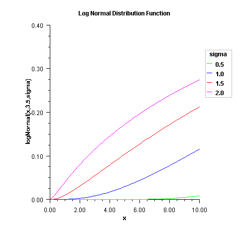
- Parameters:
x- adouble, the argument at which the function is to be evaluatedmu- adouble, the location parametersigma- adouble, the shape parameter.sigmamust be a positive.- Returns:
- a
double, the probability that a standard lognormal random variable takes a value less than or equal tox
-
generalizedExtremeValue
public static double generalizedExtremeValue(double x, double mu, double sigma, double xi) Evaluates the generalized extreme value cumulative distribution function.The cumulative distribution function for the generalized extreme value distribution is $$F(x|\mu,\sigma,\xi)=e^{-t(x)}$$ where $$t(x)=\left\{\begin{array}{lll} (1+\xi(\frac{x-\mu}{\sigma}))^{-\frac{1}{\xi}}& \mbox{for} & \xi \ne 0 \\ e^{-\frac{x-\mu}{\sigma}} & \mbox{for} & \xi = 0 \end{array}\right. $$ \( \mu\in \mathbb{R} \) is the location parameter, \(\sigma > 0 \) is the scale parameter, and \(\xi \in \mathbb{R} \) is the shape parameter. Furthermore, the support for the distribution is $$\left\{\begin{array}{lll} x \in \mathbb{R} & \mbox{for} & \xi = 0 \\ x \ge \mu - \frac{\sigma}{\xi} & \mbox{for} & \xi > 0 \\ x \le \mu - \frac{\sigma}{\xi} & \mbox{for} & \xi \lt 0 \end{array}\right. $$
- Parameters:
x- adouble, the value (quantile) at which to evaluate the cdfmu- adouble, the location parametersigma- adouble, the scale parameterxi- adouble, the shape parameter- Returns:
- a
double, the cdf evaluated atxgiven the parameter values
-
generalizedGaussian
public static double generalizedGaussian(double x, double mu, double alpha, double beta) Evaluates the generalized Gaussian (normal) cumulative distribution function.The generalized Gaussian cumulative distribution function is given by $$F(x;\mu,\alpha,\beta)=\frac{1}{2} + \frac{sign(x-\mu)}{2\Gamma(\frac{1}{\beta})} \gamma(\frac{1}{\beta},(\frac{|x-\mu|}{\alpha})^{\beta})$$ where \(\mu\) is the location parameter, \(\alpha\) is the scale parameter, \(\beta\) is the shape parameter, and \(\gamma(a,t)\) is the incomplete gamma function with shape parameter \(a\), evaluated at \(t\). Note that this follows the parameterization given in Wikipedia. There are alternative parameterizations, as in Roenko, et. al. 2014.
References
1. Roenko, Alexey, Lukin, Vladimir, Djurovic, Igor, Simeunović, Marko. (2014). Estimation of parameters for generalized Gaussian distribution. ISCCSP 2014 - 2014 6th International Symposium on Communications, Control and Signal Processing, Proceedings. 376-379.
2. Wikipedia contributors. "Generalized normal distribution." Wikipedia, The Free Encyclopedia.
- Parameters:
x- adouble, the point at which the function is to be evaluatedmu- adouble, the location parameteralpha- adouble, the scale parameter. It must be positive.beta- adouble, the shape parameter. It must be positive.- Returns:
- a
double, the probability that a generalized Gaussian random variable takes a value less than or equal tox - See Also:
-
generalizedPareto
public static double generalizedPareto(double x, double mu, double sigma, double alpha) Evaluates the generalized Pareto cumulative distribution function.The generalized Pareto cumulative distribution function is given by $$ F(x; \mu,\sigma, \alpha) =\left\{\begin{array}{cl} 1 - \left( 1 + \frac{\alpha (x-\mu)}{\sigma}\right)^{(-\frac{1}{\alpha})} & \mbox{for}~ \alpha \ne 0 \\ 1 - \exp(-\frac{x-\mu}{\sigma}) & \mbox{for}~ \alpha = 0 \end{array}\right.$$ where \(\mu \in \mathbb{R} \) is the location parameter, \(\sigma \gt 0 \) is the scale parameter, and \(\alpha \in \mathbb{R} \) is the shape parameter. The support for \(\alpha \ge 0\) is \( x \ge \mu \), while for \( \alpha \lt 0 \), \(\mu \le x \le \mu - \frac{\sigma}{\alpha}\). Note that this follows the parameterization given in Wikipedia.
References
1. Wikipedia contributors. "Generalized Pareto distribution." Wikipedia, The Free Encyclopedia.
- Parameters:
x- adouble, the point at which the function is to be evaluatedmu- adouble, the location parametersigma- adouble, the scale parameter. It must be positive.alpha- adouble, the shape parameter- Returns:
- a
double, the probability density atxgiven the parameter values
-
extremeValue
public static double extremeValue(double x, double mu, double beta) Evaluates the extreme value cumulative probability distribution function.Method
extremeValueevaluates the extreme value cumulative distribution function with location parameter \(\mu\) and shape parameter \(\beta\). The extreme value distribution, also known as the Gumbel minimum distribution, is the limiting distribution of the minimum of a large number of continuous, identically distributed random variables.$$F(x; \mu, \beta) = 1 - e^{ - e^{\frac{x-\mu}{\beta}}}$$
The case where \(\mu =0\) and \(\beta = 1\) is called the standard Gumbel distribution.
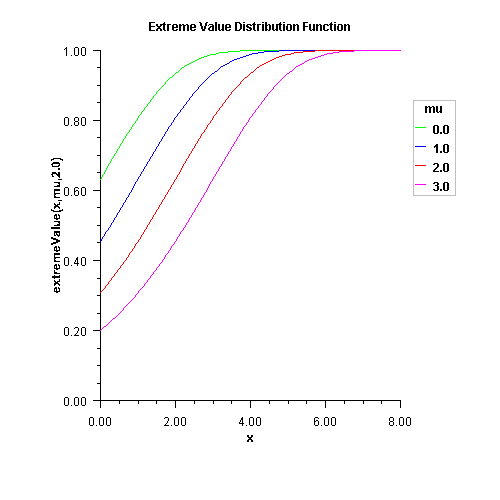
- Parameters:
x- adouble, the argument at which the function is to be evaluatedmu- adouble, the location parameter, \(\mu\)beta- adouble, the scale parameter, \(\beta\)- Returns:
- a
double, the probability that an extreme value random variable takes on a value less than or equal tox - See Also:
-
Rayleigh
public static double Rayleigh(double x, double alpha) Evaluates the Rayleigh cumulative probability distribution function.Method
Rayleighis a special case of Weibull distribution function where the shape parametergammais 2.0; that is,\(F(x) = 1-e^{-\frac{x^2}{2\alpha^2}}\)
where
alphais the scale parameter.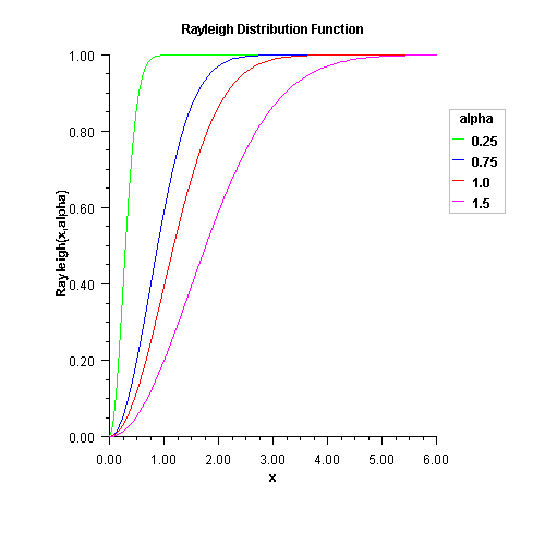
- Parameters:
x- adouble, the argument at which the function is to be evaluated. It must be non-negative.alpha- adouble, the scale parameter- Returns:
- a
double, the probability that a Rayleigh random variable takes a value less than or equal tox
-
uniform
public static double uniform(double x, double aa, double bb) Deprecated.usecontinuousUniform(double, double, double)insteadEvaluates the uniform cumulative probability distribution function.Method
$$f(x)=\left\{\begin{array}{cl} 0 & \mbox{if}~ x \lt aa \\ \frac{x-aa}{bb-aa} & \mbox{if}~ aa\le x\le bb \\ 1 &\mbox{if}~ x>bb \end{array}\right.$$uniformevaluates the distribution function, F, of a uniform random variable with location parameter aa and scale parameter bb; that is,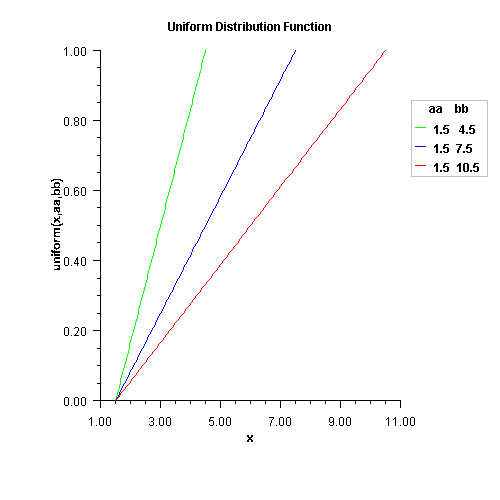
- Parameters:
x- adouble, the argument at which the function is to be evaluatedaa- adouble, the location parameterbb- adouble, the scale parameter- Returns:
- a
double, the probability that a uniform random variable takes a value less than or equal tox
-
discreteUniform
public static double discreteUniform(int x, int n) Evaluates the discrete uniform cumulative probability distribution function.- Parameters:
x- anint, the argument at which the function is to be evaluated.xshould be a value between the lower limit 0 and upper limitn.n- anint, the upper limit of the discrete uniform distribution- Returns:
- a
double, the probability that a discrete uniform random variable takes a value less than or equal tox
-
continuousUniform
public static double continuousUniform(double x, double a, double b) Evaluates the continuous uniform cumulative distribution function.The continuous uniform cumulative distribution function is $$F(x|a,b)=\left\{\begin{array}{cl} 0 & \mbox{if}~ x \lt a \\ \frac{x-a}{b-a} & \mbox{if}~ a\le x\le b \\ 1 &\mbox{if}~ x>b \end{array}\right.$$ where \( -\infty \lt a \lt b \lt \infty \).
- Parameters:
x- adouble, the value (quantile) at which to evaluate the pdfa- adouble, the lower parameter "\(a\)"b- adouble, the upper parameter "\(b\)"- Returns:
- a
double, the cumulative distribution function atxgiven the parameter values
-
geometric
public static double geometric(int x, double pin) Evaluates the discrete geometric cumulative probability distribution function.- Parameters:
x- anint, the argument at which to evaluate the functionpin- adouble, the probability of success for each independent trial- Returns:
- a
double, the probability that a geometric random variable takes a value less than or equal tox
-
logistic
public static double logistic(double x, double mu, double sigma) Evaluates the logistic cumulative probability distribution function.Method
logisticevaluates the distribution function, F, of a logistic random variable with location parameter \(\mu\) and scale parameter \(\sigma\). It is given by$$F(x,\mu,\sigma)=\frac{1}{1+e^{-(x-\mu)/\sigma}}$$
where \(\sigma>0\).
- Parameters:
x- adouble, the argument at which the function is to be evaluatedmu- adouble, the location parametersigma- adouble, the scale parameter- Returns:
- a
double, the probability that a logistic random variable takes a value less than or equal tox
-
Pareto
public static double Pareto(double x, double xm, double k) Evaluates the Pareto cumulative probability distribution function.Method
Paretoevaluates the distribution function, F, of a Pareto random variable with scale parameter \(x_m\) and shape parameter k. It is given by$$F(x,x_m,k)=1-\left ( \frac{x_m}{x} \right )^{k}$$
where \(x_m>0\) and \(k>0\). The function is only defined for \(x \geq x_m\)
- Parameters:
x- adouble, the argument at which the function is to be evaluatedxm- adouble, the scale parameter, \(x_m\)k- adouble, the shape parameter, \(k\)- Returns:
- a
double, the probability that a Pareto random variable takes a value less than or equal tox
-
binomialProb
public static double binomialProb(int k, int n, double pin) Deprecated.UsePdf.binomial(int, int, double)instead.Evaluates the binomial probability density function.Method
binomialProbevaluates the probability that a binomial random variable with parameters n and p with p=pin takes on the value k. It does this by computing probabilities of the random variable taking on the values in its range less than (or the values greater than) k. These probabilities are computed by the recursive relationship$$\Pr \left( {X = j} \right) = \frac{{\left( {n + 1 - j} \right)p}}{{j\left( {1 - p} \right)}}\Pr \left( {X = j - 1} \right)$$
To avoid the possibility of underflow, the probabilities are computed forward from 0, if k is not greater than \(n \times p\), and are computed backward from n, otherwise. The smallest positive machine number, \(\varepsilon\), is used as the starting value for computing the probabilities, which are rescaled by \((1 - p)^n \varepsilon\) if forward computation is performed and by \(p^n\varepsilon\) if backward computation is done.
For the special case of p = 0,
binomialProbis set to 0 if k is greater than 0 and to 1 otherwise; and for the case p = 1,binomialProbis set to 0 if k is less than n and to 1 otherwise.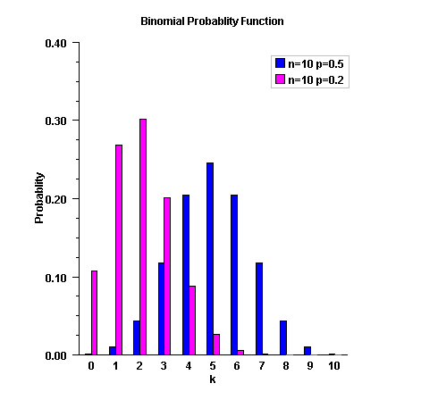
- Parameters:
k- anint, the value for which the binomial distribution function is to be evaluatedn- anint, the number of Bernoulli trialspin- adouble, the probability of success on each independent trial- Returns:
- a
double, the probability that a binomial random variable takes a value equal tok. - See Also:
-
poissonProb
public static double poissonProb(int k, double theta) Deprecated.UsePdf.poisson(int, double)instead.Evaluates the Poisson probability density function.Method
poissonProbevaluates the probability density function of a Poisson random variable with parametertheta.theta, which is the mean of the Poisson random variable, must be positive. The probability function (with \(\theta = theta\)) is$$f(x) = e^{- \theta} \,\,\theta ^k /k!,\,\,\,\,\, for\,k = 0,\,\,1,\,\,2,\, \ldots$$
poissonProbevaluates this function directly, taking logarithms and using the log gamma function.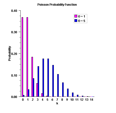
- Parameters:
k- anint, the value for which the Poisson probability function is to be evaluatedtheta- adouble, the mean of the Poisson distribution- Returns:
- a
double, the probability that a Poisson random variable takes a value equal to k - See Also:
-
betaProb
public static double betaProb(double x, double pin, double qin) Deprecated.UsePdf.beta(double, double, double)instead.Evaluates the beta probability density function.- Parameters:
x- adouble, the argument at which the function is to be evaluated.pin- adouble, the first beta distribution parameter.qin- adouble, the second beta distribution parameter.- Returns:
- a
double, the value of the probability density function atx.
-
FProb
public static double FProb(double x, double dfn, double dfd) Deprecated.UsePdf.F(double, double, double)instead.Evaluates the F probability density function.The probability density function of the F distribution is $${\it f}(x, {\it dfn}, {\it dfd})= {\frac { {\Gamma}(\frac {v_1 + v_2}{2})({\frac {v_1}{v_2})}^{\frac{v_1}{2}} x^{\frac {v_1}{2}} } {{{\Gamma}(\frac {v_1}{2}) }{{\Gamma}(\frac {v_2}{2}) } {(1+\frac{v_1x}{v_2})}^{\frac{v_1+v_2}{2} } }}$$ where \(v_1\) and \(v_2\) are the shape parameters
dfnanddfdand \(\Gamma\) is the gamma function, $${\Gamma (a)} = {\int}_{0}^{\infty}{t^{a-1} e^{-t } \it dt}$$.- Parameters:
x- adouble, the argument at which the function is to be evaluated.dfn- adouble, the numerator degrees of freedom. It must be positive.dfd- adouble, the denominator degrees of freedom. It must be positive.- Returns:
- a
double, the value of the probability density function atx.
-
hypergeometricProb
public static double hypergeometricProb(int k, int sampleSize, int defectivesInLot, int lotSize) Deprecated.UsePdf.hypergeometric(int, int, int, int)instead.Evaluates the hypergeometric probability density function.Method
hypergeometricevaluates the probability density function of a hypergeometric random variable with parameters n, l, and m. The hypergeometric random variable X can be thought of as the number of items of a given type in a random sample of size n that is drawn without replacement from a population of size l containing m items of this type. The probability density function is:$${\rm{Pr}}\left( {X = k} \right) = \frac{{\left( {_k^m } \right)\left( {_{n - k}^{l - m} } \right)}}{{\left( {_n^l } \right)}}{\rm{for}} \,\,\, k = i,\;i + 1,\,i + 2\; \ldots ,\;\min \left( {n,m} \right)$$
where i = max(0, n - l + m).
hypergeometricevaluates the expression using log gamma functions.- Parameters:
k- anint, the argument at which the function is to be evaluated.sampleSize- anint, the sample size,n.defectivesInLot- anint, the number of defectives in the lot,m.lotSize- anint, the lot size,l.- Returns:
- a
double, the probability that a hypergeometric random variable takes on a value equal tok. - See Also:
-
gammaProb
public static double gammaProb(double x, double a, double b) Deprecated.UsePdf.gamma(double, double, double)instead.Evaluates the gamma probability density function. The probability density function of the gamma distribution is$$ f(x; a, b) = x^{a - 1} \frac{1}{{b^{a} \Gamma (a)}} e^{ - {x}/{b}} $$
whereais the shape parameter andbis the scale parameter.- Parameters:
x- adouble, the argument at which the function is to be evaluated.a- adouble, the shape parameter. This must be positive.b- adouble, the scale parameter. This must be positive.- Returns:
- a
doublescalar value, the probability density function atx.
-
exponentialProb
public static double exponentialProb(double x, double scale) Deprecated.UsePdf.exponential(double, double)instead.Evaluates the exponential probability density function- Parameters:
x- adouble, the argument at which the function is to be evaluated.scale- adouble, the scale parameter.- Returns:
- a
doublescalar value, the value of the probability density function atx.
-
chiProb
public static double chiProb(double chsq, double df) Deprecated.UsePdf.chi(double, double)instead.Evaluates the chi-squared probability density function- Parameters:
chsq- adouble, the argument at which the function is to be evaluated.df- adouble, the number of degrees of freedom.dfmust be positive.- Returns:
- a
doublescalar value, the value of the probability density function atchsq.
-
WeibullProb
public static double WeibullProb(double x, double gamma, double alpha) Deprecated.UsePdf.Weibull(double, double, double)instead.Evaluates the Weibull probability density function.- Parameters:
x- adouble, the argument at which the function is to be evaluated. It must be non-negative.gamma- adouble, the shape parameter.alpha- adouble, the scale parameter.- Returns:
- a
doublescalar value, the probability density function atx.
-
logNormalProb
public static double logNormalProb(double x, double mu, double sigma) Deprecated.UsePdf.logNormal(double, double, double)instead.Evaluates the standard lognormal probability density function. $$F\left( x \right) = \frac{1}{x\sigma\sqrt{2\pi}} {e^{-\frac{ {(\ln{x}-\mu)}^2 }{2{\sigma}^2}} }$$- Parameters:
x- adouble, the argument at which the function is to be evaluated.mu- adouble, the location parameter.sigma- adouble, the shape parameter.sigmamust be a positive.- Returns:
- a
double, the probability density function atx.
-
extremeValueProb
public static double extremeValueProb(double x, double mu, double beta) Deprecated.UsePdf.extremeValue(double, double, double)instead.Evaluates the extreme value probability density function.- Parameters:
x- adouble, the argument at which the function is to be evaluated.mu- adouble, the location parameter.beta- adouble, the scale parameter.- Returns:
- a
double, the probability density function atx. - See Also:
-
RayleighProb
public static double RayleighProb(double x, double alpha) Deprecated.UsePdf.Rayleigh(double, double)instead.Evaluates the Rayleigh probability density function.- Parameters:
x- adouble, the argument at which the function is to be evaluated. It must be non-negative.alpha- adouble, the scale parameter.- Returns:
- a
double, the probability density function atx.
-
discreteUniformProb
public static double discreteUniformProb(int x, int n) Deprecated.UsePdf.discreteUniform(int, int)instead.Evaluates the discrete uniform probability density function.- Parameters:
x- anintargument for which the discrete uniform probability density function is to be evaluated.xshould be a value between the lower limit 0 and upper limitnn- anint, the upper limit of the discrete uniform distribution.- Returns:
- a
double, the probability that a discrete uniform random variable takes a value equal tox. - See Also:
-
geometricProb
public static double geometricProb(int x, double pin) Deprecated.UsePdf.geometric(int, double)instead.Evaluates the discrete geometric probability density function.Method
geometricevaluates the geometric distribution for the number of trials before the first success.- Parameters:
x- theintargument for which the geometric probability function is to be evaluatedpin- adouble, the probability parameter of the geometric distribution (the probability of success for each independent trial)- Returns:
- a
double, the probability that a geometric random variable takes a value equal tox. - See Also:
-
inverseBeta
public static double inverseBeta(double p, double pin, double qin) Deprecated.UseInvCdf.beta(double, double, double)instead.Evaluates the inverse of the beta cumulative probability distribution function.Method
inverseBetaevaluates the inverse distribution function of a beta random variable with parameterspinandqin, that is, with P = p, p = pin, and q = qin, it determines x (equal toinverseBeta (p, pin, qin)), such that$$P = \frac{{\Gamma \left( p \right)\Gamma \left( q \right)}}{{\Gamma \left( {p + q} \right)}}\int_0^x {t^{p - 1} } \left( {1 - t} \right)^{q - 1} dt$$
where \(\Gamma(\cdot)\) is the gamma function. The probability that the random variable takes a value less than or equal to x is P.
- Parameters:
p- adouble, the probability for which the inverse of the beta CDF is to be evaluated.pin- adouble, the first beta distribution parameter.qin- adouble, the second beta distribution parameter.- Returns:
- a
double, the probability that a beta random variable takes a value less than or equal to this returned value isp. - See Also:
-
inverseF
public static double inverseF(double p, double dfn, double dfd) Deprecated.UseInvCdf.F(double, double, double)instead.Returns the inverse of the F cumulative probability distribution function.Method
inverseFevaluates the inverse distribution function of a Snedecor's F random variable withdfnnumerator degrees of freedom anddfddenominator degrees of freedom. The function is evaluated by making a transformation to a beta random variable and then usinginverseBeta. If X is an F variate with \(v_1\) and \(v_2\) degrees of freedom and \(Y = v_1X/(v_2 + v_1X)\), then Y is a beta variate with parameters \(p = v_1/2\) and \(q = v_2/2\). If \(P \le 0.5\),inverseFuses this relationship directly, otherwise, it also uses a relationship between X random variables that can be expressed as follows, usingf, which is the F cumulative distribution function:$${\rm F}(X, {\it dfn}, {\it dfd})=1 - {\rm F}(1/X, {\it dfd}, {\it dfn})$$
- Parameters:
p- adouble, the probability for which the inverse of the F distribution function is to be evaluated. Argument p must be in the open interval (0.0, 1.0).dfn- adouble, the numerator degrees of freedom. It must be positive.dfd- adouble, the denominator degrees of freedom. It must be positive.- Returns:
- a
double, the probability that an F random variable takes a value less than or equal to this returned value isp. - See Also:
-
inverseGamma
public static double inverseGamma(double p, double a) Deprecated.UseInvCdf.gamma(double, double)instead.Evaluates the inverse of the gamma cumulative probability distribution function.Method
inverseGammaevaluates the inverse distribution function of a gamma random variable with shape parameter a, that is, it determines \(x ={\rm inverseGamma} (p, a))\), such that$$P = \frac{1}{{\Gamma \left( a \right)}}\int_o^x {e^{ - t} } t^{a - 1} dt$$
where \(\Gamma(\cdot)\) is the gamma function. The probability that the random variable takes a value less than or equal to x is P. See the documentation for routine
gammafor further discussion of the gamma distribution.inverseGammauses bisection and modified regula falsi to invert the distribution function, which is evaluated using methodgamma.- Parameters:
p- adouble, the probability at which the function is to be evaluated.a- adouble, the shape parameter. This must be positive.- Returns:
- a
doublescalar value. The probability that a gamma random variable takes a value less than or equal to this returned value isp. - See Also:
-
inverseNormal
public static double inverseNormal(double p) Deprecated.UseInvCdf.normal(double)instead.Evaluates the inverse of the normal (Gaussian) cumulative probability distribution function.Method
inverseNormalevaluates the inverse of the distribution function, \(\Phi\), of a standard normal (Gaussian) random variable, that is,inverseNormal\(({\rm p})=\Phi-1(p)\), where$$\Phi \left( x \right) = \frac{1}{{\sqrt {2\pi } }}\int_{ - \infty }^x {e^{ - t^2 /2} dt}$$
The value of the distribution function at the point x is the probability that the random variable takes a value less than or equal to x. The standard normal distribution has a mean of 0 and a variance of 1.
- Parameters:
p- adouble, the probability at which the function is to be evaluated.- Returns:
- a
doublescalar value. The probability that a standard normal random variable takes a value less than or equal to this returned value isp. - See Also:
-
inverseChi
public static double inverseChi(double p, double df) Deprecated.UseInvCdf.chi(double, double)instead.Evaluates the inverse of the chi-squared cumulative probability distribution function.Method
inverseChievaluates the inverse distribution function of a chi-squared random variable withdfdegrees of freedom, that is, with P = p and v = df, it determines x (equal toinverseChi(p, df)), such that$$P = \frac{1}{{2^{\nu /2} \Gamma \left( {\nu /2} \right)}}\int_0^x {e^{ - t/2} t^{\nu /2 - 1} } dt$$
where \(\Gamma(\cdot)\) is the gamma function. The probability that the random variable takes a value less than or equal to x is P.
For \(v \lt 40\),
inverseChiuses bisection, if \(v \ge 2\) or \(P \gt 0.98\), or regula falsi to find the point at which the chi-squared distribution function is equal to P. The distribution function is evaluated usingchi.For \(40 \le v \lt 100\), a modified Wilson-Hilferty approximation (Abramowitz and Stegun 1964, equation 26.4.18) to the normal distribution is used, and
inverseNormalis used to evaluate the inverse of the normal distribution function. For \(v \ge 100\), the ordinary Wilson-Hilferty approximation (Abramowitz and Stegun 1964, equation 26.4.17) is used.- Parameters:
p- adouble, the probability for which the inverse chi-squared function is to be evaluated.df- adouble, the number of degrees of freedom. This must be at least 0.5.- Returns:
- a
doublescalar value. The probability that a chi-squared random variable takes a value less than or equal to this returned value isp. - See Also:
-
inverseNoncentralchi
public static double inverseNoncentralchi(double p, double df, double alam) Deprecated.UseInvCdf.noncentralchi(double, double, double)instead.Evaluates the inverse of the noncentral chi-squared cumulative probability distribution function.Method
inverseNoncentralchievaluates the inverse distribution function of a noncentral chi-squared random variable withdfdegrees of freedom and noncentrality parameteralam, that is, with P = p, \(\nu = {\rm df}\), and \(\lambda = {\rm alam}\), it determines \(c_{0} = \)inverseNoncentralchi(p, df, alam)), such that$$P = \sum\limits_{i = 0}^\infty {\frac{e^{-\lambda/2}\left(\lambda/2\right)^i}{i!}} \int_0^{c_{0}} {\frac{x^{\left(\nu + 2i\right)/2-1}e^{ - x/2}} {2^{\left(\nu+2i\right)/2}{\Gamma\left(\frac{\nu+2i}{2}\right)}}} dx$$
where \(\Gamma (\cdot)\) is the gamma function. The probability that the random variable takes a value less than or equal to \(c_{0}\) is \(P\).
Method
inverseNoncentralchiuses bisection and modified regula falsi to invert the distribution function, which is evaluated usingnoncentralchi. Seenoncentralchifor an alternative definition of the noncentral chi-squared random variable in terms of normal random variables.- Parameters:
p- adouble, the probability for which the inverse noncentral chi-squared distribution function is to be evaluated.pmust be in the open interval (0.0, 1.0).df- adouble, the number of degrees of freedom. This must be at least 0.5. but less than or equal to 200,000.alam- adouble, the noncentrality parameter. This must be nonnegative, andalam + dfmust be less than or equal to 200,000.- Returns:
- a
doublescalar value. The probability that a noncentral chi-squared random variable takes a value less than or equal to this returned value isp. - See Also:
-
inverseStudentsT
public static double inverseStudentsT(double p, double df) Deprecated.UseInvCdf.studentsT(double, double)instead.Returns the inverse of the Student's t cumulative probability distribution function.inverseStudentsTevaluates the inverse distribution function of a Student's t random variable withdfdegrees of freedom. Let v = df. If v equals 1 or 2, the inverse can be obtained in closed form, if v is between 1 and 2, the relationship of a t to a beta random variable is exploited andinverseBetais used to evaluate the inverse; otherwise the algorithm of Hill (1970) is used. For small values of v greater than 2, Hill's algorithm inverts an integrated expansion in \(1/(1 + t^2/v)\) of the t density. For larger values, an asymptotic inverse Cornish-Fisher type expansion about normal deviates is used.- Parameters:
p- adouble, the probability for which the inverse Student's t function is to be evaluated.df- adouble, the number of degrees of freedom. This must be at least one.- Returns:
- a
doublescalar value. The probability that a Student's t random variable takes a value less than or equal to this returned value isp. - See Also:
-
inverseNoncentralstudentsT
public static double inverseNoncentralstudentsT(double p, int idf, double delta) Deprecated.UseInvCdf.noncentralstudentsT(double, int, double)instead.Evaluates the inverse of the noncentral Student's t cumulative probability distribution function.Method
inverseNoncentralstudentsTevaluates the inverse distribution function of a noncentral t random variable withidfdegrees of freedom and noncentrality parameterdelta; that is, with \(P = p\), \(\nu = idf\), \(\delta = delta\), it determines \(t_{0} = \)inverseNoncentralstudentsT(p, idf, delta)), such that$$P = \int_{-{\infty}}^{t_{0}}{\frac{\nu^{\nu/2}e^{{-\delta^2}/2}} {{\sqrt{\pi}\Gamma\left(\nu/2\right)\left(\nu+x^2\right)}^{\left(\nu+1\right)/2}} } \sum\limits_{i = 0}^\infty {\Gamma\left(\left(\nu+i+1\right)/2\right)\left(\frac{\delta^i}{i!}\right) \left(\frac{2x^2}{\nu+x^2}\right)^{i/2} dx}$$
where \(\Gamma (\cdot)\) is the gamma function. The probability that the random variable takes a value less than or equal to \(t_{0}\) is
P. SeenoncentralstudentsTfor an alternative definition in terms of normal and chi-squared random variables. The methodinverseNoncentralstudentsTuses bisection and modified regula falsi to invert the distribution function, which is evaluated usingnoncentralstudentsT.- Parameters:
p- adouble, the probability for which the function is to be evaluated.idf- anint, the number of degrees of freedom. This must be positive.delta- adouble, the noncentrality parameter.- Returns:
- a
doublescalar value. The probability that a noncentral Student's t random variable takes a value less than or equal to this returned value isp. - See Also:
-
inverseWeibull
public static double inverseWeibull(double p, double gamma, double alpha) Deprecated.UseInvCdf.Weibull(double, double, double)instead.Returns the inverse of the Weibull cumulative probability distribution function.- Parameters:
p- adouble, the probability for which the inverse Weibull function is to be evaluated.gamma- adouble, the shape parameter.alpha- adouble, the scale parameter.- Returns:
- a
doublescalar value. The probability that a Weibull random variable takes a value less than or equal to this returned value isp.
-
inverseLogNormal
public static double inverseLogNormal(double p, double mu, double sigma) Deprecated.UseInvCdf.logNormal(double, double, double)instead.Returns the inverse of the standard lognormal cumulative probability distribution function.- Parameters:
p- adouble, the probability for which the inverse lognormal function is to be evaluated.mu- adouble, the location parameter.sigma- adouble, the shape parameter.sigmamust be a positive.- Returns:
- a
doublescalar value. The probability that a standard lognormal random variable takes a value less than or equal to this returned value isp.
-
inverseExponential
public static double inverseExponential(double p, double scale) Deprecated.UseInvCdf.exponential(double, double)instead.Evaluates the inverse of the exponential cumulative probability distribution function.Method
exponentialevaluates the inverse distribution function of a gamma random variable with scale parameter =b and shape parameter a=1.0, that is, it determines \(x ={\rm exponential} (p, 1.0))\), such that$$P = \frac{1}{{\Gamma \left( a \right)}}\int_o^x {e^{ - t/b} } dt$$
where \(\Gamma(\cdot)\) is the gamma function. The probability that the random variable takes a value less than or equal to x is P. See the documentation for routine
gammafor further discussion of the gamma distribution.exponentialuses bisection and modified regula falsi to invert the distribution function, which is evaluated using methodgamma.- Parameters:
p- adouble, the probability at which the function is to be evaluated.scale- adouble, the scale parameter.- Returns:
- a
doublescalar value. The probability that an exponential random variable takes a value less than or equal to this returned value isp. - See Also:
-
inverseExtremeValue
public static double inverseExtremeValue(double p, double mu, double beta) Deprecated.UseInvCdf.extremeValue(double, double, double)instead.Returns the inverse of the extreme value cumulative probability distribution function.- Parameters:
p- adouble, the probability for which the inverse extreme value function is to be evaluated.mu- adouble, the location parameter.beta- adouble, the scale parameter.- Returns:
- a
doublescalar value. The probability that an extreme value random variable takes a value less than or equal to this returned value isp.
-
inverseRayleigh
public static double inverseRayleigh(double p, double alpha) Deprecated.UseInvCdf.Rayleigh(double, double)instead.Returns the inverse of the Rayleigh cumulative probability distribution function.- Parameters:
p- adouble, the probability for which the inverse Rayleigh function is to be evaluated.alpha- adouble, the scale parameter.- Returns:
- a
doublescalar value. The probability that a Rayleigh random variable takes a value less than or equal to this returned value isp.
-
inverseUniform
public static double inverseUniform(double p, double aa, double bb) Deprecated.UseInvCdf.uniform(double, double, double)instead.Returns the inverse of the uniform cumulative probability distribution function.- Parameters:
p- adouble, the probability for which the inverse uniform function is to be evaluated.aa- adouble, the minimum value.bb- adouble, the maximum value.- Returns:
- a
doublescalar value. The probability that a uniform random variable takes a value less than or equal to this returned value isp.
-
inverseDiscreteUniform
public static int inverseDiscreteUniform(double p, int n) Deprecated.UseInvCdf.discreteUniform(double, int)instead.Returns the inverse of the discrete uniform cumulative probability distribution function.- Parameters:
p- adouble, the probability for which the inverse discrete uniform function is to be evaluatedn- anint, the upper limit of the discrete uniform distribution- Returns:
- an
intscalar value. The probability that a discrete uniform random variable takes a value less than or equal to this returned value isp.
-
inverseGeometric
public static double inverseGeometric(double r, double pin) Deprecated.UseInvCdf.geometric(double, double)instead.Returns the inverse of the discrete geometric cumulative probability distribution function.- Parameters:
r- adouble, the probability for which the inverse geometric function is to be evaluatedpin- anint, the probability parameter for each independent trial (the probability of success for each independent trial).- Returns:
- a
doublescalar value. The probability that a geometric random variable takes a value less than or equal to this returned value is the input probability,r.
-
noncentralF
public static double noncentralF(double f, double df1, double df2, double lambda) Evaluates the noncentral F cumulative distribution function.The noncentral F distribution is a generalization of the F distribution. If \(X\) is a noncentral chi-square random variable with noncentrality parameter \(\lambda\) and \(\nu_1\) degrees of freedom, and \(Y\) is a chi-square random variable with \(\nu_2\) degrees of freedom which is statistically independent of \(X\), then $$ F \;\; = \;\; \frac{ (X/\nu_1)}{(Y/\nu_2)} $$ is a noncentral F-distributed random variable whose CDF is given by: $$ CDF(f, \nu_1, \nu_2, \lambda) \;\; = \;\; \sum_{j = 0}^\infty {c_j} $$ where: $$ c_j \;\; = \;\; \omega_j \; I_x (\frac{\nu_1}{2} + j, \; \frac{\nu_2}{2}) $$ $$ \omega_j \;\; = \;\; e^{-\lambda / 2} \; \frac{(\lambda / 2)^{j}}{j!} \;\; = \;\; \frac{\lambda}{2j} \; \omega_{j-1} $$ $$ I_x (a, b) \;\; = \;\; \frac{\beta_x (a, b)}{\beta (a, b)} $$ $$ \beta_x (a, b) \;\; = \;\; \int_{0}^{x} t^{a-1} (1-t)^{b-1} dt \;\; = \;\; x^{a} \sum_{j = 0}^\infty {\frac{\Gamma(j+1-b)} {(a+j) \; \Gamma(1-b) \; j!} \; x^{j}} $$ $$ \beta (a, b) \;\; = \;\; \beta_1 (a, b) \;\; = \;\; \frac{\Gamma(a) \; \Gamma(b)} {\Gamma(a + b)} $$ $$ I_x (a+1, b) \;\; = \;\; I_x (a, b) \; - \; T_x (a, b) $$ $$ T_x (a, b) \;\; = \;\; \frac{\Gamma(a + b)}{\Gamma(a+1) \; \Gamma(b)} x^{a} (1-x)^{b} \;\; = \;\; T_x (a-1, b) \; \frac{a-1+b}{a} \; x $$ $$ x \;\; = \;\; \frac{\nu_1 f}{\nu_2 \; + \; \nu_1 f} $$ and \(\Gamma (\cdot)\) is the gamma function, \(\nu_1\) =
df1, \(\nu_2\) =df2, \(\lambda\) =lambda, and f =f.With a noncentrality parameter of zero, the noncentral F distribution is the same as the F distribution.
- Parameters:
f- adoublevalue representing the argument at which the function is to be evaluated.fmust be nonnegative.df1- adoublevalue representing the number of numerator degrees of freedom.df1must be positive.df2- adoublevalue representing the number of denominator degrees of freedom.df2must be positive.lambda- adoublevalue representing the noncentrality parameter.lambdamust be nonnegative.- Returns:
- a
double, the probability that a noncentral F random variable takes a value less than or equal tof.
-
complementaryNoncentralF
public static double complementaryNoncentralF(double f, double df1, double df2, double lambda) Calculates the complement of the noncentral F cumulative distribution function.The complementary noncentral F distribution is a generalization of the complementary F distribution. If \(X\) is a noncentral chi-square random variable with noncentrality parameter \(\lambda\) and \(\nu_1\) degrees of freedom, and \(Y\) is a chi-square random variable with \(\nu_2\) degrees of freedom which is statistically independent of \(X\), then $$ F \;\; = \;\; \frac{ (X/\nu_1)}{(Y/\nu_2)} $$ is a noncentral F-distributed random variable whose CDF is given by: $$ F(f, \nu_1, \nu_2, \lambda) \;\; = \;\; \sum_{j = 0}^\infty {c_j} $$ where: $$ c_j \;\; = \;\; \omega_j \; I_x (\frac{\nu_1}{2} + j, \; \frac{\nu_2}{2}) $$ $$ \omega_j \;\; = \;\; e^{-\lambda / 2} \; \frac{(\lambda / 2)^{j}}{j!} \;\; = \;\; \frac{\lambda}{2j} \; \omega_{j-1} $$ $$ I_x (a, b) \;\; = \;\; \frac{\beta_x (a, b)}{\beta (a, b)} $$ $$ \beta_x (a, b) \;\; = \;\; \int_{0}^{x} t^{a-1} (1-t)^{b-1} dt \;\; = \;\; x^{a} \sum_{j = 0}^\infty {\frac{\Gamma(j+1-b)} {(a+j) \; \Gamma(1-b) \; j!} \; x^{j}} $$ $$ \beta (a, b) \;\; = \;\; \beta_1 (a, b) \;\; = \;\; \frac{\Gamma(a) \; \Gamma(b)} {\Gamma(a + b)} $$ $$ I_x (a+1, b) \;\; = \;\; I_x (a, b) \; - \; T_x (a, b) $$ $$ T_x (a, b) \;\; = \;\; \frac{\Gamma(a + b)}{\Gamma(a+1) \; \Gamma(b)} x^{a} (1-x)^{b} \;\; = \;\; T_x (a-1, b) \; \frac{a-1+b}{a} \; x $$ $$ x \;\; = \;\; \frac{\nu_1 f}{\nu_2 \; + \; \nu_1 f} $$ and \(\Gamma (\cdot)\) is the gamma function, \(\nu_1\) =
The series approximation of the complementary (cmp) noncentral F CDF, denoted by \(F(.)\), is obtainable by using the following identities: $$ \sum_{j = 0}^\infty {\omega_j} \;\; = \;\; 1 $$ $$ I_{1-x} (b, a) \;\; = \;\; 1 \; - \; I_x (a, b) $$ * $$ {\def\arraystretch{1.3}\begin{array}{ll} I_{1-x} (b, a+1) \;\; & \displaystyle = \;\; 1 \; - \; I_x (a+1, b) \;\; = \;\; 1 \; - \; I_x (a, b) \; + \; T_x (a, b) \;\; \\ & \displaystyle = \;\; I_{1-x} (b, a) \; + \; T_x (a,b) \end{array}} $$ Thus: $$ \begin{array}{ll} \overline{F}(f, \nu_1, \nu_2, \lambda) \;\; & \displaystyle = \;\; 1 \;\; - \;\; \sum_{j = 0}^\infty {c_j} \;\; = \;\; \sum_{j = 0}^\infty {\omega_j[1 \; - \; I_x (\frac{\nu_1}{2} + j, \; \frac{\nu_2}{2})]} \;\; \\ & \displaystyle = \;\; \sum_{j = 0}^\infty {\omega_j \; I_{1-x} (\frac{\nu_2}{2}, \; \frac{\nu_1}{2} + j)} \end{array} $$ We can use the above expansion of \(\overline{F}(f, \nu_1, \nu_2, \lambda)\) and the identities: $$ I_{1-x} (b, a+1) \;\; = \;\; I_{1-x} (b, a) \; + \; T_x (a, b) $$ $$ T_x (a, b) \;\; = \;\; \frac{\Gamma(a + b)}{\Gamma(a+1) \; \Gamma(b)} x^{a} (1-x)^{b} \;\; = \;\; T_x (a-1, b) \; \frac{a-1+b}{a} \; x $$ to recursively calculate \(\overline{F}(f, \nu_1, \nu_2, \lambda)\).df1, \(\nu_2\) =df2, \(\lambda\) =lambda, and f =f. The above series expansion for the noncentral F was taken from Butler and Paolella (1999) (see Paolella.pdf), with the correction for the recursion relation given below: $$ I_x\left(a+1,b\right)=I_x\left(a,b\right)-T_x\left(a,b\right) $$ extracted from the AS 63 algorithm for calculating the incomplete beta function as described by Majumder and Bhattacharjee (1973).With a noncentrality parameter of zero, the noncentral F distribution is the same as the F distribution.
- Parameters:
f- adoublevalue representing the argument at which the function is to be evaluated.fmust be nonnegative.df1- adoublevalue representing the number of numerator degrees of freedom.df1must be positive.df2- adoublevalue representing the number of denominator degrees of freedom.df2must be positive.lambda- adoublevalue representing the noncentrality parameter.lambdamust be nonnegative.- Returns:
- a
double, the probability that a noncentral F random variable takes a value greater thanf.
-
beta
public static double beta(double x, double pin, double qin) Evaluates the beta cumulative probability distribution function.Method
betaevaluates the distribution function of a beta random variable with parameterspinandqin. This function is sometimes called the incomplete beta ratio and, with p =pinand q =qin, is denoted by \(I_x(p, q)\). It is given by$$I_x \left( {p,\,q} \right) = \frac{{\Gamma \left( p \right)\Gamma \left( q \right)}}{{\Gamma \left( {p + q} \right)}}\int_0^x {\,t^{p - 1} \left( {1 - t} \right)^{q - 1} dt}$$
where \(\Gamma(\cdot)\) is the gamma function. The value of the distribution function \(I_x(p, q)\) is the probability that the random variable takes a value less than or equal to x.
The integral in the expression above is called the incomplete beta function and is denoted by \(\beta_x (p, q)\). The constant in the expression is the reciprocal of the beta function (the incomplete beta function evaluated at x=1) and is denoted by \(\beta_1 (p, q)\).
betauses the method of Bosten and Battiste (1974).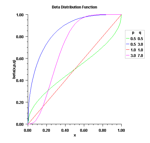
- Parameters:
x- adouble, the argument at which the function is to be evaluated.pin- adouble, the first beta distribution parameter.qin- adouble, the second beta distribution parameter.- Returns:
- a
double, the probability that a beta random variable takes on a value less than or equal tox. - See Also:
-
Pdf.beta(double, double, double)instead.