cubSplineInterpShape
Computes a shape-preserving cubic spline.
Synopsis
cubSplineInterpShape (xdata, fdata)
Required Arguments
- float
xdata[](Input) - Array with
ndatacomponents containing the abscissas of the interpolation problem. - float
fdata[](Input) - Array with
ndatacomponents containing the ordinates for the interpolation problem.
Return Value
The structure that represents the cubic spline interpolant. If an
interpolant cannot be computed, then None is returned.
Optional Arguments
concave- This option produces a cubic interpolant that will preserve the concavity of the data.
concaveItmax, int (Input)This option allows the user to set the maximum number of iterations of Newton’s Method.
Default:
concaveItmax= 25.
Description
The function cubSplineInterpShape computes a \(C^1\) cubic spline
interpolant to a set of data points \((x_i, f_i)\) for i = 0,
…, ndata − 1 = n. The breakpoints of the spline are the abscissas.
This computation is based on a method by Akima (1970) to combat wiggles in
the interpolant. Endpoint conditions are automatically determined by the
program; see Akima (1970) or de Boor (1978).
If the optional argument concave is chosen, then this function computes
a cubic spline interpolant to the data. For ease of explanation, we will
assume that \(x_i < x_{i+1}\), although it is not necessary for
the user to sort these data values. If the data are strictly convex, then
the computed spline is convex, \(C^2\), and minimizes the expression
over all convex \(C^1\) functions that interpolate the data. In the general case, when the data have both convex and concave regions, the convexity of the spline is consistent with the data, and the above integral is minimized under the appropriate constraints. For more information on this interpolation scheme, refer to Michelli et al. (1985) and Irvine et al. (1986).
One important feature of the splines produced by this function is that it is not possible, a priori, to predict the number of breakpoints of the resulting interpolant. In most cases, there will be breakpoints at places other than data locations. This function should be used when it is important to preserve the convex and concave regions implied by the data.
Both methods are nonlinear, and although the interpolant is a piecewise cubic, cubic polynomials are not reproduced. (However, linear polynomials are reproduced.) This explains the theoretical error estimate below.
If the data points arise from the values of a smooth (say \(C^4\)) function f, i.*e.* \(f_i = f(x_i)\), then the error will behave in a predictable fashion. Let ξ be the breakpoint vector for either of the above spline interpolants. Then, the maximum absolute error satisfies
where
and \(\xi_m\) is the last breakpoint.
The return value for this function is the structure Imsl_d_ppoly. This structure contains all the information to determine the spline (stored as a piecewise polynomial) that is computed by this function. For example, the following code sequence evaluates this spline at x and returns the value in y.
y = cubSplineValue (x, ppoly, 0)
The difference between the convexity-preserving spline and Akima’s spline is illustrated in the following figure. Note that the convexity-preserving interpolant exhibits linear segments where the convexity constraints are binding.
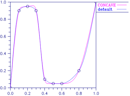
Figure 3.2 — Two Shape-Preserving Splines
Examples
Example 1
In this example, a cubic spline interpolant to a function f is computed. The values of this spline are then compared with the exact function values.
from __future__ import print_function
from numpy import *
from pyimsl.math.cubSplineInterpShape import cubSplineInterpShape
from pyimsl.math.cubSplineValue import cubSplineValue

# Define function


def F(x):
    return sin(15.0 * x)


# Compute xdata and fdata
ndata = 11
xdata = empty(ndata)
fdata = empty(ndata)
for i in range(0, ndata):
    xdata[i] = float(i) / (ndata - 1)
    fdata[i] = F(xdata[i])

# Compute cubic spline interpolant
pp = cubSplineInterpShape(xdata, fdata)

# Print results
print("   x         F(x)       Interpolant    Error")
for i in range(0, 2 * ndata - 1):
    x = float(i) / (2 * ndata - 2)
    y = cubSplineValue(x, pp)
    print('%6.3f  %10.3f   %10.3f   %10.4f' % (x, F(x), y, abs(F(x) - y)))
Output
   x         F(x)       Interpolant    Error
 0.000       0.000        0.000       0.0000
 0.050       0.682        0.818       0.1360
 0.100       0.997        0.997       0.0000
 0.150       0.778        0.615       0.1635
 0.200       0.141        0.141       0.0000
 0.250      -0.572       -0.478       0.0934
 0.300      -0.978       -0.978       0.0000
 0.350      -0.859       -0.812       0.0464
 0.400      -0.279       -0.279       0.0000
 0.450       0.450        0.386       0.0645
 0.500       0.938        0.938       0.0000
 0.550       0.923        0.854       0.0683
 0.600       0.412        0.412       0.0000
 0.650      -0.320       -0.276       0.0433
 0.700      -0.880       -0.880       0.0000
 0.750      -0.968       -0.889       0.0789
 0.800      -0.537       -0.537       0.0000
 0.850       0.183        0.149       0.0338
 0.900       0.804        0.804       0.0000
 0.950       0.994        0.932       0.0613
 1.000       0.650        0.650       0.0000
Example 2
In this example, a cubic spline interpolant to a function f is computed. The values of this spline are then compared with the exact function values.
from __future__ import print_function
from numpy import *
from pyimsl.math.cubSplineInterpShape import cubSplineInterpShape
from pyimsl.math.cubSplineValue import cubSplineValue

# Define function


def F(x):
    return sin(15.0 * x)


# Compute xdata and fdata
ndata = 11
xdata = empty(ndata)
fdata = empty(ndata)
for i in range(0, ndata):
    xdata[i] = float(i) / (ndata - 1)
    fdata[i] = F(xdata[i])

# Compute cubic spline interpolant
pp = cubSplineInterpShape(xdata, fdata, concave=True)

# Print results
print("     x         F(x)     Interpolant    Error")
for i in range(0, 2 * ndata - 1):
    x = float(i) / (2 * ndata - 2)
    y = cubSplineValue(x, pp)
    print('%6.3f  %10.3f   %10.3f   %10.4f' % (x, F(x), y, abs(F(x) - y)))
Output
     x         F(x)     Interpolant    Error
 0.000       0.000        0.000       0.0000
 0.050       0.682        0.667       0.0150
 0.100       0.997        0.997       0.0000
 0.150       0.778        0.761       0.0172
 0.200       0.141        0.141       0.0000
 0.250      -0.572       -0.559       0.0126
 0.300      -0.978       -0.978       0.0000
 0.350      -0.859       -0.840       0.0189
 0.400      -0.279       -0.279       0.0000
 0.450       0.450        0.440       0.0098
 0.500       0.938        0.938       0.0000
 0.550       0.923        0.902       0.0208
 0.600       0.412        0.412       0.0000
 0.650      -0.320       -0.311       0.0086
 0.700      -0.880       -0.880       0.0000
 0.750      -0.968       -0.952       0.0156
 0.800      -0.537       -0.537       0.0000
 0.850       0.183        0.200       0.0174
 0.900       0.804        0.804       0.0000
 0.950       0.994        0.892       0.1020
 1.000       0.650        0.650       0.0000
Warning Errors
IMSL_MAX_ITERATIONS_REACHED |
The maximum number of iterations has been reached. The best approximation is returned. |
Fatal Errors
IMSL_DUPLICATE_XDATA_VALUES |
The xdata values must be distinct. |