cubSplineTcb¶

Computes a tension-continuity-bias (TCB) cubic spline interpolant. This is also called a Kochanek-Bartels spline and is a generalization of the Catmull–Rom spline.

Synopsis¶

cubSplineTcb (xdata, fdata)

Required Arguments¶

float xdata[] (Input): Array with ndata components containing the abscissas of the interpolation problem.
float fdata[] (Input): Array with ndata components containing the ordinates for the interpolation problem.

Return Value¶

The structure that represents the interpolant. If an interpolant cannot be computed, None is returned.

Optional Arguments¶

tension, float[] (Input)

Sets the tension values at the data points. The array tension is of length ndata and contains tension values in the interval [-1,1]. For each point, if the tension value is near +1 the curve is tightened at that point. If it is near -1, the curve is slack.

Default: All values of tension are zero.

continuity, float[] (Input)

Sets the continuity values at the data points. The array continuity is of length ndata and contains continuity values in the interval [-1,1]. For each point, if the continuity value is zero the curve is \(C^1\) at that point. Otherwise the curve has a corner at that point, but is still continuous (\(C^0\)).

Default: All values of continuity are zero.

bias, float[] (Input)

Sets the bias values at the data points. The array bias is of length ndata and contains bias values in the interval [-1,1]. For each point, if the bias value is zero the left and right side tangents are equally weighted. If the value is near +1 the left-side tangent dominates. If the value is near -1 the right-side tangent dominates.

Default: All values of bias are zero.

left, float (Input)

Sets the value of the tangent at the leftmost endpoint.

Default: left = 0.

right, float (Input)

Sets the value of the tangent at the rightmost endpoint.

Default: right = 0.

Description¶

The function cubSplineTcb computes the Kochanek-Bartels spline, a piecewise cubic Hermite spline interpolant to a set of data points \(\{x_i, f_i\}\) for I = 0, …, ndata-1. The breakpoints of the spline are the abscissas. As with all of the univariate interpolation functions, the abscissas need not be sorted.

The \(\{x_i\}\) values are the knots, so the i-th interval is \(\left[x_i, x_{i+1}\right]\). (To simplify the explanation, it is assumed that the data points are given in increasing order.) The cubic Hermite in the i-th segment has a starting value of \(f_i\) and an ending value of \(f_{i+1}\). Its incoming tangent is

\[DS_i = \frac{1}{2}\left(1-t_i\right)\left(1-c_i\right)\left(1+b_i\right)\frac{y_i-y_{i-1}}{x_{i+1}-x_i} + \frac{1}{2}\left(1-t_i\right)\left(1+c_i\right)\left(1-b_i\right)\frac{y_{i+1} - y_i}{x_{i+1} - x_i}\]

where \(t_i\) is the i-th tension value, \(c_i\) is the i-th continuity value, and \(b_i\) is the i-th bias value. Its outgoing tangent is

\[DD_i = \frac{1}{2}\left(1-t_i\right)\left(1+c_i\right)\left(1+b_i\right)\frac{y_i-y_{i-1}}{x_{i+1}-x_i} + \frac{1}{2}\left(1-t_i\right)\left(1-c_i\right)\left(1-b_i\right)\frac{y_{i+1} - y_i}{x_{i+1} - x_i}\]

The optional arguments left and right are used at the endpoints:

\[\frac{y_0-y_{-1}}{x_1-x_o} = \mathit{left}\]

and

\[\frac{y_n-y_{n-1}}{x_n-x_{n-1}} = \mathrm{right}\]

Both left and right default to zero.

The spline has a continuous first derivative (is \(C^1\)) if at each data point the left and right tangents are equal. This is true if the continuity parameters, \(c_i\), are all zero. For any values of the parameters the spline is continuous (\(C^0\)).

If \(t_i = c_i = b_i = 0\) for all i, then the curve is the Catmull-Rom spline.

The following chart shows the same data points interpolated with different parameter values. All of the tension, continuity and bias parameters are zero except for the labeled parameter, which has the indicated value at all data points.

Tension controls how sharply the spline bends at the data points. If tension is near +1, the curve tightens. If tension is near -1, the curve slackens.

The continuity parameter controls the continuity of the first derivative. If continuity is zero, the spline’s first derivative is continuous, so the spline is \(C^1\).

The bias parameter controls the weighting of the left and right tangents. If zero, the tangents are equally weighted. If the bias parameter is near +1, the left tangent dominates. If the bias parameter is near -1, the right tangent dominates.

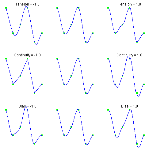
../../_images/Figure-InterpolatedDataPoints.png

Figure 3.3 — Data Points Interpolated with Different Parameter Values

Examples¶

Example 1¶

This example interpolates to a set of points. At \(x = 3\) the continuity and tension parameters are -1. At all other points, they are zero. Interpolated values are then printed.

from __future__ import print_function
from numpy import *
from pyimsl.math.cubSplineTcb import cubSplineTcb
from pyimsl.math.cubSplineValue import cubSplineValue

xdata = [0, 1, 2, 3, 4, 5]
fdata = [5, 2, 3, 5, 1, 2]
continuity = [0, 0, 0, -1, 0, 0]
tension = [0, 0, 0, -1, 0, 0]
m = 2

ppoly = cubSplineTcb(xdata, fdata,
                     continuity=continuity,
                     tension=tension)

for i in range(0, m * len(xdata) - 1):
    x = float(i) / m
    y = cubSplineValue(x, ppoly)
    print(" %6.3f %10.4f" % (x, y))

Output¶

000     5.0000
500     3.4375
000     2.0000
500     2.1875
000     3.0000
500     3.6875
000     5.0000
500     2.1875
000     1.0000
500     1.2500
000     2.0000

Example 2¶

It is possible to use an interpolating spline for approximation by using an optimization function to compute its parameters. In this example a series of n interest rates, \(r_i\), for different maturities, \(x_i\), is given, \(\{x_i, r_i\}\) for \(i = 0, …, n-1\). Since the dates are given on a widely varying time scale, the base 10 logarithm of the dates is used for interpolation.

A TCB spline is constructed using a subset of the given data points for knot locations, \(\{p_i, q_i\}\), for \(i = 0, …, m-1\). The p values are a subset of the \(log_{10}x_i\) values. The q values are to be determined by the optimizer. The spline has non-zero values of the continuity parameter, \(c_i\), for \(i = 0, …, m-1\).

The optimization problem finds the spline, \(s\left( r_i; p, q, c, \mathit{left}, \mathit{right} \right)\) , which interpolates the points \(\{p_i, q_i\}\) and has continuity parameters, c, and specified left and right parameters.

The optimization problem is

\[\min_{q,c,\mathit{left},\mathit{right}} \textstyle\sum_{i=0}^{i=n-1} \left| s\left(r_i;q,c,\mathit{left},\mathit{right}\right) - r_i \right|^2\]

subject to the bounds, for all i.

\[0.1 \leq q_i \leq 10\]

\[-0.95 \leq c_i \leq 0.95\]

The function constrainedNlp is used as the optimizer. The unknowns q, c, left and right are packed into the array x, respectively.

from __future__ import print_function
from numpy import *
from pyimsl.math.cubSplineTcb import cubSplineTcb
from pyimsl.math.cubSplineValue import cubSplineValue
from pyimsl.math.constrainedNlp import constrainedNlp

N_DATA = 15
days = array([3, 31, 62, 94, 185, 367, 731, 1096, 1461, 1826, 2194,
              2558, 2922, 3287, 3653])
rate = array([5.01772, 4.98284, 4.97234, 4.96157, 4.99058,
              5.09389, 5.79733, 6.30595, 6.73464, 6.94816, 7.08807, 7.27527,
              7.30852, 7.3979, 7.49015])

# Knots are set on a subset of the data points
N_KNOTS = 4
subset = [0, 5, 10, 14]

xknots = zeros(N_KNOTS)
Y_KNOTS = 0
CONTINUITY = Y_KNOTS + N_KNOTS
LEFT = CONTINUITY + N_KNOTS
RIGHT = LEFT + 1
N_VARIABLES = RIGHT + 1

# Function passed to imsl_d_constrained_nlp


def fcn(n, x, iact, result, ierr):
    if (iact == 0):
        result[0] = objective(
            x[Y_KNOTS:N_KNOTS], x[CONTINUITY:CONTINUITY + N_KNOTS], x[LEFT], x[RIGHT])
    return

# Compute the objective function, the sum of squares error


def objective(yknots, continuity, left, right):
    ppoly = cubSplineTcb(xknots, yknots,
                         continuity=continuity,
                         left=left,
                         right=right)

    error = 0.0
    for i in range(0, N_DATA):
        y = cubSplineValue(log_days[i], ppoly)
        diff = (y - rate[i])
        error += diff * diff
    return error / N_DATA


# Note: xlb and xub need to be List variables when passed to constrainedNlp
xlb = list(range(0, N_VARIABLES))
xub = list(range(0, N_VARIABLES))
xguess = zeros(N_VARIABLES)
n_constraints = 0
ibtype = 0
for i in range(0, N_KNOTS):
    xlb[Y_KNOTS + i] = 0.1       # lower bound on rate
    xub[Y_KNOTS + i] = 10.0      # upper bound on rate
    xlb[CONTINUITY + i] = -0.95  # lower bound on continuity
    xub[CONTINUITY + i] = 0.95   # upper bound on continuity

# Set bounds wide enough on LEFT and RIGHT so they are not binding
xlb[LEFT] = -100.0
xub[LEFT] = 100.0
xlb[RIGHT] = -100.0
xub[RIGHT] = 100.0

log_days = zeros(len(days))
for i in range(0, N_DATA):
    log_days[i] = log10(days[i])

for i in range(0, N_KNOTS):
    xknots[i] = log_days[subset[i]]
    xguess[Y_KNOTS + i] = rate[subset[i]]
    xguess[CONTINUITY + i] = 0.0

xguess[LEFT] = xguess[RIGHT] = 0.0

# Find the optimial curve
x = constrainedNlp(fcn, n_constraints, 0, ibtype, xlb, xub,
                   xguess=xguess,
                   difftype=3)

# Report results
ppoly = cubSplineTcb(xknots, x[0:N_KNOTS],
                     continuity=x[CONTINUITY:CONTINUITY + N_KNOTS])

print("Days  Rate   Curve  Error")
for i in range(0, N_DATA):
    y = cubSplineValue(log_days[i], ppoly)
    print("%4d %6.3f %6.3f %6.3f" % (days[i], rate[i], y, y - rate[i]))
print()
for i in range(0, N_KNOTS):
    print("  continuity[%2d] = %6.3f" % (days[i], x[CONTINUITY + i]))
print("\n  left  = %6.3f\n  right = %6.3f" % (x[LEFT], x[RIGHT]))

Output¶

Days  Rate   Curve  Error
   3  5.018  5.019  0.002
  31  4.983  4.926 -0.057
  62  4.972  4.911 -0.061
  94  4.962  4.919 -0.043
 185  4.991  4.970 -0.021
 367  5.094  5.084 -0.010
 731  5.797  5.842  0.045
1096  6.306  6.340  0.034
1461  6.735  6.683 -0.052
1826  6.948  6.931 -0.017
2194  7.088  7.118  0.030
2558  7.275  7.240 -0.035
2922  7.309  7.332  0.023
3287  7.398  7.409  0.011
3653  7.490  7.479 -0.011

  continuity[ 3] =  0.009
  continuity[31] = -0.630
  continuity[62] = -0.184
  continuity[94] = -0.950

  left  =  0.534
  right =  0.266