nonlinLeastSquares

Solves a nonlinear least-squares problem using a modified Levenberg-Marquardt algorithm.

Synopsis

nonlinLeastSquares (fcn, m, n)

Required Arguments

void fcn (m, n, x[], f[]) (Input/Output)

User-supplied function to evaluate the function that defines the least-squares problem where x is a vector of length n at which point the function is evaluated, and f is a vector of length m containing the function values at point x.

int m (Input)

Number of functions.

int n (Input)

Number of variables where n ≤ m.

Return Value

The solution x of the nonlinear least-squares problem. If no solution can be computed, then None is returned.

Optional Arguments

xguess, float[] (Input)

Array with n components containing an initial guess.

Default: xguess = 0

jacobian, void jacobian (m, n, x[], fjac[]) (Input)

User-supplied function to compute the Jacobian where x is a vector of length n at which point the Jacobian is evaluated, fjac is the computed m × n Jacobian at the point x.

Note that each derivative \(\partial f_i/\partial x_j\) should be returned in fjac[(i-1)]

xscale, float[] (Input)

Array with n components containing the scaling vector for the variables. xscale is used mainly in scaling the gradient and the distance between two points. See keywords gradTol and stepTol for more detail.

Default: xscale[] = 1.

fscale, float[] (Input)

Array with m components containing the diagonal scaling matrix for the functions. The i-th component of fscale is a positive scalar specifying the reciprocal magnitude of the i-th component function of the problem.

Default: fscale[] = 1.

gradTol, float (Input)

Scaled gradient tolerance. The i-th component of the scaled gradient at x is calculated as

\[\frac {\left|g_i\right| * \max\left(\left|x_i\right|, 1/s_i\right)} {\tfrac{1}{2}\left\|F(x)\right\|_2^2}\]

where \(g=\nabla F(x)\), s = xscale, and

\[\left\|F(x)\right\|_2^2 = \textstyle\sum_{i=1}^{m} f_i(x)^2\]

Default: gradTol = \(\sqrt{\varepsilon}\), \(\sqrt[3]{\varepsilon}\) in double where ɛ is the machine precision.

stepTol, float (Input)

Scaled step tolerance. The i-th component of the scaled step between two points x and y is computed as

\[\frac{\left|x_i-y_y\right|}{\max\left(\left|x_i\right|, 1/s_i\right)}\]

where s = xscale.

Default: stepTol = \(\varepsilon^{2/3}\) where ɛ is the machine precision.

relFcnTol, float (Input)

Relative function tolerance.

Default: relFcnTol = \(\max(10^{-10} \varepsilon^{2/3})\), \(\max (10^{-20},\varepsilon^{2/3})\) in double, where ɛ is the machine precision

absFcnTol, float (Input)

Absolute function tolerance.

Default: absFcnTol = \(\max(10^{-20},\varepsilon^2)\), \(\max(10^{-40},\varepsilon^2)\) in double, where ɛ is the machine precision.

maxStep, float (Input)

Maximum allowable step size.

Default: maxStep = \(1000 \max(\varepsilon_1,\varepsilon_2)\) where,

\[\varepsilon_1 = \left( \textstyle\sum_{i=1}^{n} \left(s_it_i\right)^2 \right)^{1/2}, \varepsilon_2 = \|s\|_2\]

s = xscale, and t = xguess

initTrustRegion, float (Input)

Size of initial trust region radius. The default is based on the initial scaled Cauchy step.

goodDigit, int (Input)

Number of good digits in the function.

Default: machine dependent.

maxItn, int (Input)

Maximum number of iterations.

Default: maxItn = 100.

maxFcn, int (Input)

Maximum number of function evaluations.

Default: maxFcn = 400.

maxJacobian, int (Input)

Maximum number of Jacobian evaluations.

Default: maxJacobian = 400.

internScale

Internal variable scaling option. With this option, the values for xscale are set internally.

tolerance, float (Input)

The tolerance used in determining linear dependence for the computation of the inverse of \(J^T J\). For nonlinLeastSquares, if jacobian is specified, then tolerance = 100 × machine(4) is the default. Otherwise, the square root of machine(4) is the default. For nonlinLeastSquares, if jacobian is specified, then tolerance = 100 × machine(4) is the default. Otherwise, the square root of machine(4) is the default. See machine.

fvec (Output)

A real array of length m containing the residuals at the approximate solution. On return, the necessary space is allocated by nonlinLeastSquares.

fjac (Output)

An array of size m × n containing the Jacobian at the approximate solution. On return, the necessary space is allocated by nonlinLeastSquares.

rank (Output)

The rank of the Jacobian is returned in rank.

jtjInverse, float jtjInverse (Output)

An array of size n × n containing the inverse matrix of \(J^T J\) where the J is the final Jacobian. If \(J^T J\) is singular, the inverse is a symmetric \(g_2\) inverse of \(J^T J\). (See linSolNonnegdef in Linear Systemsfor a discussion of generalized inverses and definition of the \(g_2\) inverse.) On return, the necessary space is allocated by nonlinLeastSquares.

Description

The function nonlinLeastSquares is based on the MINPACK routine LMDER by Moré et al. (1980). It uses a modified Levenberg-Marquardt method to solve nonlinear least-squares problems. The problem is stated as follows:

\[\min\tfrac{1}{2} F(x)^T F(x) = \tfrac{1}{2} \sum_{i=1}^{m} f_i(x)^2\]

where \(m\geq n\), \(F : \Re^n\rightarrow Re^m\), and \(f_i(x)\) is the i-th component function of \(F(x)\). From a current point, the algorithm uses the trust region approach,

\[\begin{split}\begin{array}{l} \min\limits_{x \in R^n} \left\|F\left(x_c\right) + J\left(x_c\right)\left(x_n-x_c\right)\right\|_2 \\ \text{subject to } \left\|x_n-x_c\right\|_2 \leq \delta_c \end{array}\end{split}\]

to get a new point \(x_n\), which is computed as

\[x_n = x_c − (J(x_c)^T J(x_c) + μ_cI)^{-1} J(x_c)^T F(x_c)\]

where \(\mu_c\) = 0 if \(\delta_c\geq\|(J(x_c)^T J(x_c))^{-1} J(x_c)^T F(x_c)\|_2\) and \(\mu_c>0\), otherwise. The value \(\mu_c\) is defined by the function. The vector and matrix \(F(x_c)\) and \(J(x_c)\) are the function values and the Jacobian evaluated at the current point \(x_c\), respectively. This function is repeated until the stopping criteria are satisfied.

The first stopping criterion for nonlinLeastSquares occurs when the norm of the function is less than the absolute function tolerance absFcnTol. The second stopping criterion occurs when the norm of the scaled gradient is less than the given gradient tolerance gradTol. The third stopping criterion for nonlinLeastSquares occurs when the scaled distance between the last two steps is less than the step tolerance stepTol. For more details, see Levenberg (1944), Marquardt (1963), or Dennis and Schnabel (1983, Chapter 10).

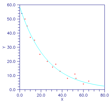
Figure 8.7 — Plot of the Nonlinear Fit

Examples

Example 1

In this example, the nonlinear data-fitting problem found in Dennis and Schnabel (1983, p. 225),

\[\min \frac{1}{2} \sum_{i=1}^{3} f_i(x)^2\]

where

\[f_i(x) = e^{t_ix} - y_i\]

is solved with the data \(t=(1,2,3)\) and \(y=(2,4,3)\).

from numpy import *
from pyimsl.math.nonlinLeastSquares import nonlinLeastSquares
from pyimsl.math.writeMatrix import writeMatrix


# Function to solve
def fcn(m, n, x, f):
    y = [2.0, 4.0, 3.0]
    t = [1.0, 2.0, 3.0]
    for i in range(0, m):
        f[i] = exp(x[0] * t[i]) - y[i]


m = 3
n = 1
fx = empty(3, dtype='double')

result = nonlinLeastSquares(fcn, m, n)
fcn(m, n, result, fx)

# Print results
writeMatrix("The solution is ", result)
writeMatrix("The function values are ", fx)

Output

 
The solution is 
          0.44
 
      The function values are 
          1            2            3
     -0.447       -1.589        0.744

Example 2

In this example, nonlinLeastSquares is first invoked to fit the following nonlinear regression model discussed by Neter et al. (1983, pp. 475-478):

\[y_i = \theta_1 e^{\theta_2 x_i} + \varepsilon_i \phantom{...} i=1,2,\ldots 15\]

where the \(\varepsilon_i\)’s are independently distributed each normal with mean zero and variance \(\sigma^2\). The estimate of \(\sigma^2\) is then computed as

\[s^2 = \frac{\sum_{i=1}^{15} e_i^2}{15 - \mathrm{rank}(J)}\]

where \(e_i\) is the i-th residual and J is the Jacobian. The estimated asymptotic variance-covariance matrix of \(\hat{\theta}_1\) and \(\hat{\theta}_2\) is computed as

\[\mathit{est.asy.var}\left(\hat{\theta}\right) = s^2\left(J^TJ\right)^{-1}\]

Finally, the diagonal elements of this matrix are used together with tInverseCdf (see Chapter 9, Special Functions) to compute 95% confidence intervals on \(\theta_1\) and \(\theta_2\).

from __future__ import print_function
from numpy import *
from pyimsl.math.nonlinLeastSquares import nonlinLeastSquares
from pyimsl.math.tInverseCdf import tInverseCdf
from pyimsl.math.writeMatrix import writeMatrix


# Function to solve
def fcn2(m, n, x, f):
    y = [54.0, 50.0, 45.0, 37.0, 35.0, 25.0, 20.0, 16.0,
         18.0, 13.0, 8.0, 11.0, 8.0, 4.0, 6.0]
    xdata = [2.0, 5.0, 7.0, 10.0, 14.0, 19.0, 26.0, 31.0,
             34.0, 38.0, 45.0, 52.0, 53.0, 60.0, 65.0]
    for i in range(0, m, 1):
        f[i] = y[i] - x[0] * exp(x[1] * xdata[i])


m = 15
n = 2
xguess = [60.0, -0.03]
e = []
rank = []
jtjInv = []

result = nonlinLeastSquares(fcn2, m, n,
                            xguess=xguess,
                            gradTol=1.0e-3,
                            fvec=e,
                            rank=rank,
                            jtjInverse=jtjInv)
dfe = double(m - rank[0])
s2 = 0.0
for i in range(0, m):
    s2 = s2 + e[i] * e[i]
s2 = s2 / dfe
j = n * n
for i in range(0, n):
    for j in range(0, n):
        jtjInv[i][j] = s2 * jtjInv[i][j]

fmt = "%15.5e"
writeMatrix("Estimated Asymptotic Variance-Covariance Matrix",
            jtjInv, writeFormat=fmt)
print("\n           95%% Confidence Intervals   ")
print("   Estimate  Lower Limit  Upper Limit ")
for i in range(0, n):
    a = tInverseCdf(0.975, dfe) * sqrt(jtjInv[i][i])
    print("  %10.3f %12.3f %12.3f"
          % (result[i], result[i] - a, result[i] + a))

Output

           95%% Confidence Intervals   
   Estimate  Lower Limit  Upper Limit 
      58.607       55.426       61.787
      -0.040       -0.043       -0.036
 
Estimated Asymptotic Variance-Covariance Matrix
                       1                2
      1      2.16726e+00     -1.78152e-03
      2     -1.78152e-03      2.92853e-06

Informational Errors

IMSL_STEP_TOLERANCE

Scaled step tolerance satisfied. The current point may be an approximate local solution, but it is also possible that the algorithm is making very slow progress and is not near a solution, or that stepTol is too big.

Warning Errors

IMSL_LITTLE_FCN_CHANGE	Both the actual and predicted relative reductions in the function are less than or equal to the relative function tolerance.
IMSL_TOO_MANY_ITN	Maximum number of iterations exceeded.
IMSL_TOO_MANY_FCN_EVAL	Maximum number of function evaluations exceeded.
IMSL_TOO_MANY_JACOBIAN_EVAL	Maximum number of Jacobian evaluations exceeded.
IMSL_UNBOUNDED	Five consecutive steps have been taken with the maximum step length.

Fatal Errors

IMSL_FALSE_CONVERGE	The iterates appear to be converging to a noncritical point.
IMSL_STOP_USER_FCN	Request from user supplied function to stop algorithm. User flag = “#”.