kohonenSOMTrainer

Trains a Kohonen network.
Synopsis
kohonenSOMTrainer (fcn, lcn, nrow, ncol, data)
Required Arguments
- float
fcn(intnrow, intncol, inttotalIter, intt, floatd) (Input/Output) User-supplied neighborhood function. In the simplest form, the neighborhood function h(d, t) is 1 for all nodes closest to the BMU and 0 for others, but a Gaussian function is also commonly used. For example:
\[h(d,t) = e^{^{-d^2}\!/_{2r^2}}\]where r represents the neighborhood radius at index t
Arguments
- int
nrow(Input) - The number of rows in the node grid.
- int
ncol(Input) - The number of columns in the node grid.
- int
totalIter(Input) - The number of iterations for training.
- int
t(Input) - The current iteration of the training.
- float
d(Input) - The lattice distance between the best matching node and the current node.
Return Value
The computed neighborhood function value.
- int
- float
lcn(intnrow, intncol, inttotalIter, intt) (Input/Output) User supplied learning coefficient function. The monotonically decreasing learning coefficient function α(t) is a scalar factor that defines the size of the update correction. The value of α(t) decreases with the step index t. Typical forms are linear, power, and inverse time/step. For example:
power:
\[\alpha(t) = \alpha_0 \left( \tfrac{\alpha_T}{\alpha_0} \right)^{^t\!/_T}\]where t=
t, T=totalIter, \(\alpha_0\) = initial learning coefficient, \(\alpha_T\) = final learning coefficientinverse time:
\[\alpha(t) = \tfrac{\mathrm{A}}{t + \mathrm{B}}\]where A and B are user determined constants
Arguments
- int
nrow(Input) - The number of rows in the node grid.
- int
ncol(Input) - The number of columns in the node grid.
- int
totalIter(Input) - The number of iterations for training.
- int
t(Input) - The current iteration of the training.
- Return Value
- The computed learning coefficient.
- int
- int
nrow(Input) - The number of rows in the node grid.
nrowmust be greater than zero. - int
ncol(Input) - The number of columns in the node grid.
ncolmust be greater than zero. - float
data[[]](Input) - An
nObs×dimarray containing the data to be used for training the Kohonen network.
Return Value
A Imsls_d_kohonenSOM data structure containing the trained Kohonen
network. Please see Data Structures for a
description of this data structure.
Optional Arguments
rectangular, (Input)- Specifies a rectangular grid should be used. Optional Arguments
rectangularandhexagonalare mutually exclusive.
Argument |
Action |
|---|---|
rectangular |
Use a rectangular grid. |
hexagonal |
Use a hexagonal grid. |
Default: A rectangular grid is used.
or
hexagonal- Specifies a hexagonal grid should be used. Optional Arguments
rectangularandhexagonalare mutually exclusive.
Argument |
Action |
|---|---|
rectangular |
Use a rectangular grid. |
hexagonal |
Use a hexagonal grid. |
Default: A rectangular grid is used.
vonNeumann, (Input)Use the Von Neumann neighborhood type. Optional Arguments
vonNeumannandmooreare mutually exclusive.ArgumentAction vonNeumannUse the Von Neumann neighborhood type. mooreUse the Moore neighborhood type. Default: The Von Neumann neighborhood type is used.
or
moore- Use the Moore neighborhood type. Optional Arguments
vonNeumannandmooreare mutually exclusive.
Argument |
Action |
|---|---|
vonNeumann |
Use the Von Neumann neighborhood type. |
moore |
Use the Moore neighborhood type. |
Default: The Von Neumann neighborhood type is used.
wrapAround, (Input)Wrap around the opposite edges. A hexagonal grid must have an even number of rows to wrap around.
Default: Do not wrap around the opposite edges.
randomSeed, int (Input)The seed of the random number generator used in generating the initial weights. If
randomSeedis 0, a value is computed using the system clock; hence, the results may be different between different calls with the same input.Default:
randomSeed= 0.iterations, int (Input)The number of iterations to be used for training.
Default:
iterations= 100.initialWeights, float[](Input)The initial weights of the nodes.
Default: Initial weights are generated internally using random uniform number generator.
reconstructionError(Output)- The sum of the Euclidean distance between the input,
data, and the nodes in the trained Kohonen network.
Description
A self-organizing map (SOM), also known as a Kohonen map or Kohonen SOM, is a technique for gathering high-dimensional data into clusters that are constrained to lie in low dimensional space, usually two dimensions. A Kohonen map is a widely used technique for the purpose of feature extraction and visualization for very high dimensional data in situations where classifications are not known beforehand. The Kohonen SOM is equivalent to an artificial neural network having inputs linked to every node in the network. Self-organizing maps use a neighborhood function to preserve the topological properties of the input space.
In a Kohonen map, nodes are arranged in a rectangular or hexagonal grid or lattice. The input is connected to each node, and the output of the Kohonen map is the zero-based (i, j) index of the node that is closest to the input. A Kohonen map involves two steps: training and forecasting. Training builds the map using input examples (vectors), and forecasting classifies a new input.
During training, an input vector is fed to the network. The input’s Euclidean distance from all the nodes is calculated. The node with the shortest distance is identified and is called the Best Matching Unit, or BMU. After identifying the BMU, the weights of the BMU and the nodes closest to it in the SOM lattice are updated towards the input vector. The magnitude of the update decreases with time and with distance (within the lattice) from the BMU. The weights of the nodes surrounding the BMU are updated according to:
where \(W_t\) represents the node weights, α(t) is the monotonically decreasing learning coefficient function, h(d,*t*) is the neighborhood function, d is the lattice distance between the node and the BMU, and \(D_t\) is the input vector.
The monotonically decreasing learning coefficient function α(t) is a scalar factor that defines the size of the update correction. The value of α(t) decreases with the step index t.
The neighborhood function h(d,*t*) depends on the lattice distance d between the node and the BMU, and represents the strength of the coupling between the node and BMU. In the simplest form, the value of h(d,*t*) is 1 for all nodes closest to the BMU and 0 for others, but a Gaussian function is also commonly used. Regardless of the functional form, the neighborhood function shrinks with time (Hollmén, 15.2.1996). Early on, when the neighborhood is broad, the self-organizing takes place on the global scale. When the neighborhood has shrunk to just a couple of nodes, the weights converge to local estimates.
Note that in a rectangular grid, the BMU has four closest nodes for the Von Neumann neighborhood type, or eight closest nodes for the Moore neighborhood type. In a hexagonal grid, the BMU has six closest nodes.
During training, this process is repeated for a number of iterations on all input vectors.
During forecasting, the node with the shortest Euclidean distance is the winning node, and its (i, j) index is the output.
Data Structures
| Field | Description |
|---|---|
int
grid |
0 = rectangular grid. Otherwise, hexagonal grid. |
int
type |
0 = Von Neumann neighborhood type. Otherwise, Moore neighborhood type. |
int
wrap |
0 = do not wrap-around node edges. Otherwise, wrap-around node edges. |
int
dim |
Number of weights in each node. |
int
nrow |
Number of rows in the node grid. |
int
ncol |
Number of columns in the node grid. |
float
weights |
Array of length nrow × ncol × dim
containing the weights of the nodes. |
Example
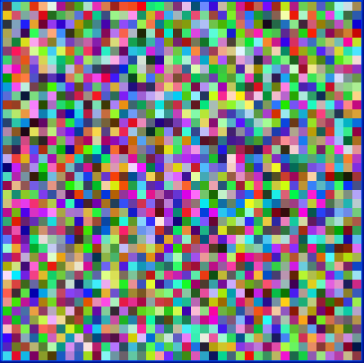
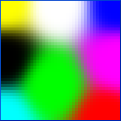
This example creates a Kohonen network with 40 × 40 nodes. Each node has three weights, representing the RGB values of a color. This network is trained with eight colors using 500 iterations. Then, the example prints out a forecast result. Initially, the image of the nodes is:

After the training, the image is:

from __future__ import print_function
from numpy import *
from pyimsl.stat.kohonenSOMTrainer import kohonenSOMTrainer
from pyimsl.stat.kohonenSOMForecast import kohonenSOMForecast


def fcn(nRow, nCol, totalIter, t, d):
    maximum = max(nRow, nCol)
    # A Gaussian function
    factor = maximum / 4.0
    c = float(totalIter - t) / float(totalIter / factor)
    return exp(-(d * d) / (2.0 * c * c))


def lcn(nRow, nCol, totalIter, t):
    initialLearning = 0.07
    return initialLearning * exp(-(float(t)) / (float(totalIter)))


nRow = 40
nCol = 40
data = [[1.0, 0.0, 0.0],
        [0.0, 1.0, 0.0],
        [0.0, 0.0, 1.0],
        [1.0, 1.0, 0.0],
        [1.0, 0.0, 1.0],
        [0.0, 1.0, 1.0],
        [0.0, 0.0, 0.0],
        [1.0, 1.0, 1.0]]
forecasts = []
fData = [[0.25, .5, 0.75]]
reconstructionError = []
error = []

kohonen = kohonenSOMTrainer(fcn, lcn, nRow, nCol, data,
                            randomSeed=123457, iterations=500,
                            reconstructionError=error)

forecasts = kohonenSOMForecast(kohonen, fData)
print("The output node is at (%d, %d)."
      % (forecasts[0][0], forecasts[0][1]))
print("Reconstruction error is %f" % error[0])
Output
The output node is at (25, 11).
Reconstruction error is 13589.442143