autocorrelation¶

Computes the sample autocorrelation function of a stationary time series.

Synopsis¶

autocorrelation (x, lagmax)

Required Arguments¶

float x[] (Input): Array of length nObservations containing the time series.
int lagmax (Input): Maximum lag of autocovariance, autocorrelations, and standard errors of autocorrelations to be computed. lagmax must be greater than or equal to 1 and less than nObservations.

Return Value¶

An array of length lagmax + 1 containing the autocorrelations of the time series x. The 0-th element of this array is 1. The k-th element of this array contains the autocorrelation of lag k where k = 1, …, lagmax.

Optional Arguments¶

printLevel, int (Input)

Printing option.

`printLevel`	Action
0	No printing is performed.
1	Prints the mean and variance.
2	Prints the mean, variance, and autocovariances.
3	Prints the mean, variance, autocovariances, autocorrelations, and standard errors of autocorrelations.

Default = 0.

acv (Output)

An array of length lagmax + 1 containing the variance and autocovariances of the time series x. The 0-th element of this array is the variance of the time series x. The k-th element contains the autocovariance of lag k where k = 1, …, lagmax.

seac, float standardErrors, int seOption (Output)

An array of length lagmax containing the standard errors of the autocorrelations of the time series x.

Method of computation for standard errors of the autocorrelations is chosen by seOption.

`seOption`	Action
`1`	Compute the standard errors of `autocorrelations` using Barlett’s formula.
2	Compute the standard errors of autocorrelations using Moran’s formula.

Description¶

Function autocorrelation estimates the autocorrelation function of a stationary time series given a sample of n = nObservations observations \(\{X_t\}\) for \(t=1,2,\ldots,n\).

Let \(\hat{\mu}\) be the estimate of the mean μ of the time series \(\{X_t\}\) where

\[\begin{split}\hat{\mu} = \begin{cases} \mu, & \mu \text{ known (xMeanIn)} \\ \frac{1}{n} \sum\limits_{t=1}^{n} X_t & \mu \text{ unknown (xMeanOut)} \\ \end{cases}\end{split}\]

The autocovariance function σ(k) is estimated by

\[\hat{\sigma}(k) = \frac{1}{n} \sum_{t=1}^{n-k} \left(X_t - \hat{\mu}\right)\left(X_{t+k} - \hat{\mu}\right), \phantom{...} k=0,1,\ldots,K\]

where K = lagmax. Note that

\[\hat{\sigma}(0)\]

is an estimate of the sample variance. The autocorrelation function ρ(k) is estimated by

\[\hat{\rho}(k) = \frac{\hat{\sigma}(k)}{\hat{\sigma}(0)}, \phantom{...} k = 0,1,\ldots,K\]

Note that

\[\hat{\rho}(0) \equiv 1\]

by definition.

The standard errors of the sample autocorrelations may be optionally computed according to argument seOption for the optional argument seac. One method (Bartlett 1946) is based on a general asymptotic expression for the variance of the sample autocorrelation coefficient of a stationary time series with independent, identically distributed normal errors. The theoretical formula is

\[\text{var}\left\{\hat{\rho}(k)\right\} = \frac{1}{n} \sum_{i = -\infty}^{\infty} \left[ \rho^2(i) + \rho(i - k)\rho(i + k) - 4\rho(i)\rho(k)\rho(i - k) + 2\rho^2(i)\rho^2(k) \right]\]

where

\[\hat{\rho}(k)\]

assumes μ is unknown. For computational purposes, the autocorrelations r(k) are replaced by their estimates

\[\hat{\rho}(k)\]

for \(|k|\leq K\), and the limits of summation are bounded because of the assumption that \(r(k)=0\) for all k such that \(|k|>K\).

A second method (Moran 1947) utilizes an exact formula for the variance of the sample autocorrelation coefficient of a random process with independent, identically distributed normal errors. The theoretical formula is

\[\mathrm{var}\left\{\hat{\rho}(k)\right\} = \frac{n-k}{n(n+2)}\]

where μ is assumed to be equal to zero. Note that this formula does not depend on the autocorrelation function.

Example¶

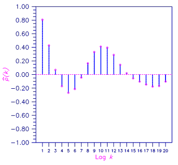
Consider the Wolfer Sunspot Data (Anderson 1971, page 660) consisting of the number of sunspots observed each year from 1749 through 1924. The data set for this example consists of the number of sunspots observed from 1770 through 1869. Function autocorrelation with optional arguments computes the estimated autocovariances, estimated autocorrelations, and estimated standard errors of the autocorrelations.

from __future__ import print_function
from numpy import *
from pyimsl.stat.autocorrelation import autocorrelation
from pyimsl.stat.dataSets import dataSets

x = empty(100)
xmean = []
nobs = 100
lagmax = 20
acv = []
seac = {'seOption': 1}

data = dataSets(2)
for i in range(0, nobs):
    x[i] = data[21 + i][1]

result = autocorrelation(x, lagmax,
                         xMeanOut=xmean,
                         acv=acv,
                         seac=seac)

print("Mean     = %8.3f" % xmean[0])
print("Variance = %8.1f" % acv[0])
print("\nLag\t   ACV\t\t   AC\t\t   SEAC\n")
print("%2d\t%8.1f\t%8.5f" % (0, acv[0], result[0]))
for i in range(1, 21):
    print("%2d\t%8.1f\t%8.5f\t%8.5f" %
          (i, acv[i], result[i], seac['standardErrors'][i - 1]))

Output¶

Mean     =   46.976
Variance =   1382.9

Lag	   ACV		   AC		   SEAC

 1382.9	 1.00000
 1115.0	 0.80629	 0.03478
  592.0	 0.42809	 0.09624
   95.3	 0.06891	 0.15678
 -236.0	-0.17062	 0.20577
 -370.0	-0.26756	 0.23096
 -294.3	-0.21278	 0.22899
  -60.4	-0.04371	 0.20862
  227.6	 0.16460	 0.17848
  458.4	 0.33146	 0.14573
  567.8	 0.41061	 0.13441
  546.1	 0.39491	 0.15068
  398.9	 0.28848	 0.17435
  197.8	 0.14300	 0.19062
   26.9	 0.01945	 0.19549
  -77.3	-0.05588	 0.19589
 -143.7	-0.10394	 0.19629
 -202.0	-0.14610	 0.19602
 -245.4	-0.17743	 0.19872
 -230.8	-0.16691	 0.20536
 -142.9	-0.10332	 0.20939

Figure 8.3 — Sample Autocorrelation Function