Neural Networks – An Overview
Today, neural networks are used to solve a wide variety of problems, some of which have been solved by existing statistical methods, and some of which have not. These applications fall into one of the following three categories:
Forecasting, pattern recognition and classification problems are not new. They existed years before the discovery of neural network solutions in the 1980’s. What is new is that neural networks provide a single framework for solving so many traditional problems and, in some cases, extend the range of problems that can be solved.
Traditionally, these problems were solved using a variety of widely known statistical methods:
In many cases, simple neural network configurations yield the same solution as many traditional statistical applications. For example, a single-layer, feedforward neural network with linear activation for its output perceptron is equivalent to a general linear regression fit. Neural networks can provide more accurate and robust solutions for problems where traditional methods do not completely apply.
Mandic and Chambers (2001) identify the traditional methods for time series forecasting that are unsuitable when a time series:
ARIMA and other traditional time series approaches can produce poor forecasts when one or more of the above conditions exist. The forecasts of ARMA and non-linear ARMA (NARMA) depend heavily upon key assumptions about the model or underlying relationship between the output of the series and its patterns.
Neural networks, on the other hand, adapt to changes in a non-stationary series and can produce reliable forecasts even when the series contains a good deal of noise or when only a short series is available for training. Neural networks provide a single tool for solving many problems traditionally solved using a wide variety of statistical tools and for solving problems when traditional methods fail to provide an acceptable solution.
Although neural network solutions to forecasting, pattern recognition and classification problems can vary vastly, they are always the result of computations that proceed from the network inputs to the network outputs. The network inputs are referred to as patterns, and outputs are referred to as classes. Frequently the flow of these computations is in one direction, from the network input patterns to its outputs. Networks with forward-only flow are referred to as feedforward networks.
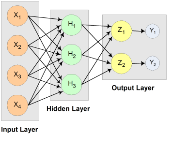
Figure 23, A 2-layer, Feedforward Network with 4 inputs and 2 outputs
Other networks, such as recurrent neural networks, allow data and information to flow in both directions, see Mandic and Chambers (2001).
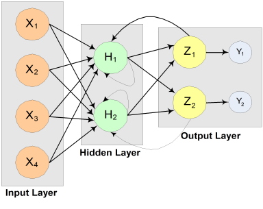
Figure 24, A recurrent neural network with 4 inputs and 2 outputs
A neural network is defined not only by its architecture and flow, or interconnections, but also by computations used to transmit information from one node or input to another node. These computations are determined by network weights. The process of fitting a network to existing data to determine these weights is referred to as training the network, and the data used in this process are referred to as patterns. Individual network inputs are referred to as attributes and outputs are referred to as classes. The table below lists terms used to describe neural networks that are synonymous to common statistical terminology.
Neural Network Terminology | Traditional Statistical Terminology | Description |
|---|---|---|
Training | Model Fitting | Estimating unknown parameters or coefficients in the analysis |
Patterns | Cases or Observations | A single observation of all input and output variables |
Attributes | Independent Variables | Inputs to the network or model |
Classes | Dependent Variables | Outputs from the network or model calculations |
Neural Networks – History and Terminology
The Threshold Neuron
McCulloch and Pitts’ (1943) wrote one of the first published works on neural networks. This paper describes the threshold neuron as a model for which the human brain stores and processes information.
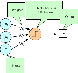
Figure 25, The McCulloch and Pitts’ Threshold Neuron
All inputs to a threshold neuron are combined into a single number, Z, using the following weighted sum:
Where m is the number of inputs and is the weight associated with the i-th input (attribute) . The term μ in this calculation is referred to as the bias term. In traditional statistical terminology it might be referred to as the intercept. The weights and bias terms in this calculation are estimated during network training.
In McCulloch and Pitts’ (1943) description of the threshold neuron, the neuron does not respond to its inputs unless Z is greater than zero. If Z is greater than zero then the output from this neuron is set to 1. If Z is less than or equal to zero the output is zero:
where Y is the neuron’s output.
Years following McCulloch and Pitts’ (1943) article, interest in McCulloch and Pitts’ neural network was limited to theoretical discussions, such as Hebb (1949), which describe learning, memory and the brain’s structure.
The Perceptron
The McCulloch and Pitts’ neuron is also referred to as a threshold neuron since it abruptly changes its output from 0 to 1 when its potential, Z, crosses a threshold. Mathematically, this behavior can be viewed as a step function that maps the neuron’s potential, Z, to the neuron’s output, Y.
Rosenblatt (1958) extended the McCulloch and Pitts’ threshold neuron by replacing this step function with a continuous function that maps Z to Y. The Rosenblatt neuron is referred to as the perceptron, and the continuous function mapping Z to Y makes it easier to train a network of perceptrons than a network of threshold neurons.
Unlike the threshold neuron, the perceptron produces analog output rather than the threshold neuron’s purely binary output. Carefully selecting the analog function, makes Rosenblatt’s perceptron differentiable, whereas the threshold neuron is not. This simplifies the training algorithm.
Like the threshold neuron, Rosenblatt’s perceptron starts by calculating a weighted sum of its inputs,
This is referred to as the perceptron’s potential.
Rosenblatt’s perceptron calculates its analog output from its potential. There are many choices for this calculation. The function used for this calculation is referred to as the activation function as shown in Figure 26 below.
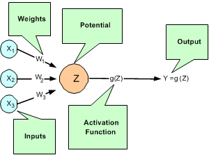
Figure 26, A Neural Net Perceptron
As shown in Figure 26, perceptrons consist of the following five components:
1. Inputs – x1, x2, and x3,
2. Input Weights – W1, W2, and W3,
3. Potential – , where μ is a bias correction,
4. Activation Function – g(Z), and
5. Output – Y = g(Z) .
Like threshold neurons, perceptron inputs can be either the initial raw data inputs or the output from another perceptron. The primary purpose of network training is to estimate the weights associated with each perceptron’s potential. The activation function maps this potential to the perceptron’s output.
The Activation Function
Although theoretically any differentiable function can be used as an activation function, the identity and sigmoid functions are the two most commonly used.
The identity activation function, also referred to as a linear activation function, is a flow-through mapping of the perceptron’s potential to its output:
Output perceptrons in a forecasting network often use the identity activation function.

Figure 27, An Identity (Linear) Activation Function
If the identity activation function is used throughout the network, then it is easily shown that the network is equivalent to fitting a linear regression model of the form , where are the k network inputs, is the i-th network output and are the coefficients in the regression equation. As a result, it is uncommon to find a neural network with identity activation used in all its perceptrons.
Sigmoid activation functions are differentiable functions that map the perceptron’s potential to a range of values, such as 0 to 1, i.e., ℝk→ℝ where K is the number of perceptron inputs.

Figure 28, A Sigmoid Activation Function
In practice, the most common sigmoid activation function is the logistic function that maps the potential into the range 0 to 1:
Since 0 < g(Z) < 1, the logistic function is very popular for use in networks that output probabilities.
Other popular sigmoid activation functions include:
It is easy to show that the hyperbolic-tangent and logistic activation functions are linearly related. Consequently, forecasts produced using logistic activation should be close to those produced using hyperbolic-tangent activation. However, one function may be preferred over the other when training performance is a concern. Researchers report that the training time using the hyperbolic-tangent activation function is shorter than using the logistic activation function.
Network Applications
Forecasting using Neural Networks
There are numerous good statistical forecasting tools. Most require assumptions about the relationship between the variables being forecasted and the variables used to produce the forecast, as well as the distribution of forecast errors. Such statistical tools are referred to as parametric methods. ARIMA time series models, for example, assume that the time series is stationary, that the errors in the forecasts follow a particular ARIMA model, and that the probability distribution for the residual errors is Gaussian, see Box and Jenkins (1970). If these assumptions are invalid, then ARIMA time series forecasts can be substandard.
Neural networks, on the other hand, require few assumptions. Since neural networks can approximate highly non-linear functions, they can be applied without an extensive analysis of underlying assumptions.
Another advantage of neural networks over ARIMA modeling is the number of observations needed to produce a reliable forecast. ARIMA models generally require 50 or more equally spaced, sequential observations in time. In many cases, neural networks can also provide adequate forecasts with fewer observations by incorporating exogenous, or external, variables in the network’s input.
For example, a company applying ARIMA time series analysis to forecast business expenses would normally require each of its departments, and each sub-group within each department, to prepare its own forecast. For large corporations this can require fitting hundreds or even thousands of ARIMA models. With a neural network approach, the department and sub-group information could be incorporated into the network as exogenous variables. Although this can significantly increase the network’s training time, the result would be a single model for predicting expenses within all departments.
Linear least squares models are also popular statistical forecasting tools. These methods range from simple linear regression for predicting a single quantitative outcome to logistic regression for estimating probabilities associated with categorical outcomes. It is easy to show that simple linear least squares forecasts and logistic regression forecasts are equivalent to a feedforward network with a single layer. For this reason, single-layer feedforward networks are rarely used for forecasting. Instead multilayer networks are used.
Hutchinson (1994) and Masters (1995) describe using multilayer feedforward neural networks for forecasting. Multilayer feedforward networks are characterized by the forward-only flow of information in the network. The flow of information and computations in a feedforward network is always in one direction, mapping an M-dimensional vector of inputs to a C-dimensional vector of outputs, i.e., where .
There are many other types of networks without this feed forward requirement. Information and computations in a recurrent neural network, for example, flows in both directions. Output from one level of a recurrent neural network can be fed back, with some delay, as input into the same network (see Figure 24). Recurrent networks are very useful for time series prediction, see Mandic and Chambers (2001).
Pattern Recognition using Neural Networks
Neural networks are also extensively used in statistical pattern recognition. Pattern recognition applications that make wide use of neural networks include:
The interest in pattern recognition using neural networks has stimulated the development of important variations of feedforward networks. Two of the most popular are:
Useful mathematical descriptions of the neural network methods underlying these applications are given by Bishop (1995), Ripley (1996), Mandic and Chambers (2001), and Abe (2001). From a statistical viewpoint, Warner and Misra (1996) describes an excellent overview of neural networks.
Neural Networks for Classification
Classifying observations using prior concomitant information is possibly the most popular application of neural networks. Data classification problems abound in business and research. When decisions based upon data are needed, they can often be treated as a neural network data classification problem. Decisions to buy, sell, or hold a stock are decisions involving three choices. Classifying loan applicants as good or bad credit risks, based upon their application, is a classification problem involving two choices. Neural networks are powerful tools for making decisions or choices based upon data.
These same tools are ideally suited for automatic selection or decision-making. Incoming email, for example, can be examined to separate spam from important email using a neural network trained for this task. A good overview of solving classification problems using multilayer feedforward neural networks is found in Abe (2001) and Bishop (1995).
There are two popular methods for solving data classification problems using multilayer feedforward neural networks, depending upon the number of choices (classes) in the classification problem. If the classification problem involves only two choices, then it can be solved using a neural network with a single logistic output. This output estimates the probability that the input data belong to one of the two choices.
For example, a multilayer feedforward network with a single logistic output can be used to determine whether a new customer is credit-worthy. The network’s input would consist of information on the applicants credit application, such as age, income, etc. If the network output probability is above some threshold value (such as 0.5 or higher) then the applicant’s credit application is approved. This is referred to as binary classification using a multilayer feedforward neural network.
If more than two classes are involved then a different approach is needed. A popular approach is to assign logistic output perceptrons to each class in the classification problem. The network assigns each input pattern to the class associated with the output perceptron that has the highest probability for that input pattern. However, this approach produces invalid probabilities since the sum of the individual class probabilities for each input is not equal to one, which is a requirement for any valid multivariate probability distribution.
To avoid this problem, the softmax activation function, see Bridle (1990), applied to the network outputs ensures that the outputs conform to the mathematical requirements of multivariate classification probabilities. If the classification problem has C categories, or classes, then each category is modeled by one of the network outputs. If Zi is the weighted sum of products between its weights and inputs for the i-th output, i.e.,
then
The softmax activation function ensures that all outputs conform to the requirements for multivariate probabilities. That is, 0 < softmaxi < 1, for all i = 1, 2, …, C and
A pattern is assigned to the i-th classification when softmaxi is the largest among all C classes.
However, multilayer feedforward neural networks are only one of several popular methods for solving classification problems. Others include:
Support Vector Machines are simple modifications of traditional multilayer feedforward neural networks (MLFF) configured for pattern classification.


