Multilayer Feedforward Neural Networks
A multilayer feedforward neural network is an interconnection of perceptrons in which data and calculations flow in a single direction, from the input data to the outputs. The number of layers in a neural network is the number of layers of perceptrons. The simplest neural network is one with a single input layer and an output layer of perceptrons. The network in Figure 13-7 illustrates this type of network. Technically, this is referred to as a one-layer feedforward network with two outputs because the output layer is the only layer with an activation calculation.
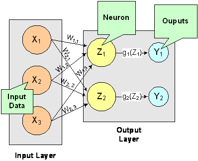
Figure 29, A Single-Layer Feedforward Neural Net
In this single-layer feedforward neural network, the network’s inputs are directly connected to the output layer perceptrons, Z1 and Z2.
The output perceptrons use activation functions, g1 and g2, to produce the outputs Y1 and Y2.
Since
and
When the activation functions g1 and g2 are identity activation functions, the single-layer neural network is equivalent to a linear regression model. Similarly, if g1 and g2 are logistic activation functions, then the single-layer neural network is equivalent to logistic regression. Because of this correspondence between single-layer neural networks and linear and logistic regression, single-layer neural networks are rarely used in place of linear and logistic regression.
The next most complicated neural network is one with two layers. This extra layer is referred to as a hidden layer. In general there is no restriction on the number of hidden layers. However, it has been shown mathematically that a two-layer neural network can accurately reproduce any differentiable function, provided the number of perceptrons in the hidden layer is unlimited.
However, increasing the number of perceptrons increases the number of weights that must be estimated in the network, which in turn increases the execution time for the network. Instead of increasing the number of perceptrons in the hidden layers to improve accuracy, it is sometimes better to add additional hidden layers, which typically reduce both the total number of network weights and the computational time. However, in practice, it is uncommon to see neural networks with more than two or three hidden layers.
Neural Network Error Calculations
Error Calculations for Forecasting
The error calculations used to train a neural network are very important. Researchers have investigated many error calculations in an effort to find a calculation with a short training time appropriate for the network’s application. Typically, error calculations are very different depending primarily on the network’s application.
For forecasting, the most popular error function is the sum-of-squared errors, or one of its scaled versions. This is analogous to using the minimum least squares optimization criterion in linear regression. Like least squares, the sum-of-squared errors is calculated by looking at the squared difference between what the network predicts for each training pattern and the target value, or observed value, for that pattern. Formally, the equation is the same as one-half the traditional least squares error:
where N is the total number of training cases, C is equal to the number of network outputs, is the observed output for the i-th training case and the j-th network output, and is the network’s forecast for that case.
Common practice recommends fitting a different network for each forecast variable. That is, the recommended practice is to use C=1 when using a multilayer feedforward neural network for forecasting. For classification problems with more than two classes, it is common to associate one output with each classification category, i.e., C=number of classes.
Notice that in ordinary least squares, the sum-of-squared errors are not multiplied by one-half. Although this has no impact on the final solution, it significantly reduces the number of computations required during training.
Also note that as the number of training patterns increases, the sum-of-squared errors increases. As a result, it is often useful to use the root-mean-square (RMS) error instead of the unscaled sum-of-squared errors:
where is the average output:
Unlike the unscaled sum-of-squared errors, ERMS does not increase as N increases. The smaller values for ERMS, indicate that the network predicts its training targets closer. The smallest value, ERMS =0, indicates that the network predicts every training target exactly. The largest value, ERMS =1, indicates that the network predicts the training targets only as well as setting each forecast equal to the mean of the training targets.
Notice that the root-mean-squared error is related to the sum-of-squared error by a simple scale factor:
Another popular error calculation for forecasting from a neural network is the Minkowski-R error. The sum-of-squared error, E, and the root-mean-squared error, ERMS, are both theoretically motivated by assuming the noise in the target data is Gaussian. In many cases, this assumption is invalid. A generalization of the Gaussian distribution to other distributions gives the following error function, referred to as the Minkowski-R error:
Notice that ER=2E when R =2.
A good motivation for using ER instead of E is to reduce the impact of outliers in the training data. The usual error measures, E and ERMS, emphasize larger differences between the training data and network forecasts since they square those differences. If outliers are expected, then it is better to de-emphasize larger differences. This can be done by using the Minkowski-R error with R =1. When R =1, the Minkowski-R error simplifies to the sum of absolute differences:
L is also referred to as the Laplacian error. This name is derived from the fact that it can be theoretically justified by assuming the noise in the training data follows a Laplacian, rather than Gaussian, distribution.
Of course, similar to E, L generally increases when the number of training cases increases. Similar to ERMS, a scaled version of the Laplacian error can be calculated using the following formula:
Cross-Entropy Error for Binary Classification
As previously mentioned, multilayer feedforward neural networks can be used for both forecasting and classification applications. Training a forecasting network involves finding the network weights that minimize either the Gaussian or Laplacian distributions, E or L, respectively, or equivalently their scaled versions, ERMSor LRMS. Although these error calculations can be adapted for use in classification by setting the target classification variable to zeros and ones, this is not recommended. Use of the sum-of-squared and Laplacian error calculations is based on the assumption that the target variable is continuous. In classification applications, the target variable is a discrete random variable with C possible values, where C = number of classes.
A multilayer feedforward neural network for classifying patterns into one of only two categories is referred to as a binary classification network. It has a single output: the estimated probability that the input pattern belongs to one of the two categories. The probability that it belongs to the other category is equal to one minus this probability, i.e., P(C2) = P(not C1) = 1-P(C1).
Binary classification applications are very common. Any problem requiring yes/no classification is a binary classification application. For example, deciding to sell or buy a stock is a binary classification problem. Deciding to approve a loan application is also a binary classification problem. Deciding whether to approve a new drug or to provide one of two medical treatments are binary classification problems.
For binary classification problems, only a single output is used, C =1. This output represents the probability that the training case should be classified as “yes.” A common choice for the activation function of the output of a binary classification network is the logistic activation function, which always results in an output in the range 0 to 1, regardless of the perceptron’s potential.
One choice for training binary classification networks is to use sum-of-squared errors with the class value of yes patterns coded as a 1 and the no classes coded as a 0, i.e.:
However, using either the sum-of-squared or Laplacian errors for training a network with these target values assumes that the noise in the training data are Gaussian. In binary classification, the zeros and ones are not Gaussian. They follow the Bernoulli distribution:
where p is equal to the probability that a randomly selected case belongs to the “yes” class.
Modeling the binary classes as Bernoulli observations leads to the use of the cross-entropy error function described by Hopfield (1987) and Bishop (1995):
where N is the number of training patterns, is the target value for the i-th case (either 1 or 0), and is the network output for the i-th training pattern. This is equal to the neural network’s estimate of the probability that the i-th training pattern should be classified as “yes.”
For situations in which the target variable is a probability in the range , the value of the cross-entropy at the network’s optimum is equal to:
Subtracting from gives an error term bounded below by zero, i.e.,
where
This adjusted cross-entropy, , is normally reported when training a binary classification network where . Otherwise , the unadjusted cross-entropy error, is used. For , small values, i.e. values near zero, indicate that the training resulted in a network able to classify the training cases with a low error rate.
Cross-Entropy Error for Multiple Classes
Using a multilayer feedforward neural network for binary classification is relatively straightforward. A network for binary classification only has a single output that estimates the probability that an input pattern belongs to the “yes” class, i.e., . In classification problems with more than two mutually exclusive classes, the calculations and network configurations are not as simple.
One approach is to use multiple network outputs, one for each of the C classes. Using this approach, the j-th output for the i-th training pattern, , is the estimated probability that the i-th pattern belongs to the j-th class, denoted by . An easy way to estimate these probabilities is to use logistic activation for each output. This ensures that each output satisfies the univariate probability requirements, i.e., .
However, since the classification categories are mutually exclusive, each pattern can only be assigned to one of the C classes, which means that the sum of these individual probabilities should always equal 1. Yet, if each output is the estimated probability for that class, it is very unlikely that
In fact, the sum of the individual probability estimates can easily exceed 1 if logistic activation is applied to every output.
Support Vector Machine (SVM) neural networks use this approach with one modification. An SVM network classifies a pattern as belonging to the i-th category if the activation calculation for that category exceeds a threshold and the other calculations do not exceed this value. That is, the i-th pattern is assigned to the j-th category if and only if and for all , where δ is the threshold. If this does not occur, then the pattern is marked as unclassified.
Another approach to multiclass classification problems is to use the softmax activation function developed by Bridle (1990) on the network outputs. This approach produces outputs that conform to the requirements of a multinomial distribution. That is
and
The softmax activation function estimates classification probabilities using the following softmax activation function:
where is the potential for the j-th output perceptron, or category, using the i-th pattern.
For this activation function, it is clear that:
Modeling the C network outputs as multinomial observations leads to the cross-entropy error function described by Hopfield (1987) and Bishop (1995):
where N is the number of training patterns, is the target value for the j-th class of i-th pattern (either 1 or 0), and is the network’s j-th output for the i-th pattern. is equal to the neural network’s estimate of the probability that the i-th pattern should be classified into the j-th category.
For situations in which the target variable is a probability in the range , the value of the cross-entropy at the networks optimum is equal to:
Subtracting this from EC gives an error term bounded below by zero, i.e., ECE ≥ 0 where:
This adjusted cross-entropy is normally reported when training a binary classification network where 0 < tij < 1. Otherwise EC, the non-adjusted cross-entropy error, is used. That is, when 1-in-C encoding of the target variable is used,
Small values, values near zero, indicate that the training resulted in a network with a low error rate and that patterns are being classified correctly most of the time.
Back-Propagation in Multilayer Feedforward Neural Networks
Sometimes a multilayer feedforward neural network is referred to incorrectly as a back-propagation network. The term back-propagation does not refer to the structure or architecture of a network. Back-propagation refers to the method used during network training. More specifically, back-propagation refers to a simple method for calculating the gradient of the network, that is the first derivative of the weights in the network.
The primary objective of network training is to estimate an appropriate set of network weights based upon a training dataset. Many ways have been researched for estimating these weights, but they all involve minimizing some error function. In forecasting the most commonly used error function is the sum-of-squared errors:
Training uses one of several possible optimization methods to minimize this error term. Some of the more common are: steepest descent, quasi-Newton, conjugant gradient and many various modifications of these optimization routines.
Back-propagation is a method for calculating the first derivative, or gradient, of the error function required by some optimization methods. It is certainly not the only method for estimating the gradient. However, it is the most efficient. In fact, some will argue that the development of this method by Werbos (1974), Parker (1985) and Rumelhart, Hinton and Williams (1986) contributed to the popularity of neural network methods by significantly reducing the network training time and making it possible to train networks consisting of a large number of inputs and perceptrons. Function imsls_f_mlff_network_trainer Stage I training is implemented using Quasi-Newton optimization and steepest ascent with gradients estimated using the back-propagation method. Stage II training is implemented using Quasi-Newton optimization.
Simply stated, back-propagation is a method for calculating the first derivative of the error function with respect to each network weight. Bishop (1995) derives and describes these calculations for the two most common forecasting error functions – the sum-of-squared errors and Laplacian error functions. Abe (2001) gives the description for the classification error function - the cross-entropy error function. For all of these error functions, the basic formula for the first derivative of the network weight wji at the i-th perceptron applied to the output from the j-th perceptron is:
where is the output from the i-th perceptron after activation, and
is the derivative for a single output and a single training pattern. The overall estimate of the first derivative of wji is obtained by summing this calculation over all N training patterns and C network outputs.
The term back-propagation gets its name from the way the term δj in the back-propagation formula is calculated:
where the summation is over all perceptrons that use the activation from the j-th perceptron, g(aj).
The derivative of the activation functions, g' (aj), varies among these functions. See the following table:
Activation Function | g(a) | g’(a) |
|---|---|---|
Linear | ||
Logistic | ||
Hyperbolic-tangent | ||
Squash |


