Synopsis with Optional Arguments
#include <imsls.h>
float *imsls_f_mlff_initialize_weights (Imsls_f_NN_Network *network, int n_patterns, int n_nominal, int n_continuous, int nominal[], float continuous[],
IMSLS_METHOD, int method,
IMSLS_PRINT,
IMSLS_CLASSIFICATION, int classification[],
IMSLS_RETURN_USER, float weights[],
0)
Optional Arguments
IMSLS_METHOD, int method (Input)
Specifies the algorithm to use for initializing weights. method contains the weight initialization method to be used. Valid values for method are:
Specifies the algorithm to use for initializing weights. method contains the weight initialization method to be used. Valid values for method are:
method | Algorithm |
|---|---|
IMSLS_EQUAL | Equal weights |
IMSLS_RANDOM | Random Weights |
IMSLS_PRINCIPAL_COMPONENTS | Principal Component Weights |
IMSLS_DISCRIMINANT | Discriminant Analysis Weights |
The discriminant weights method can only be used to initialize weights for classification networks without binary encoded nominal attributes. See the Description section for details.
Default: method = IMSLS_RANDOM.
IMSLS_PRINT, (Input)
Initial weights are printed.
Initial weights are printed.
Default: No printing is performed.
IMSLS_CLASSIFICATION, int classification[] (Input)
An array of length n_patterns containing the encoded training target classifications which must be integers from 0 to n_classes-1. Here n_classes =network‑ >n_outputs except when n_outputs=1 then n_classes =2. classification[i] is the target classification for the i-th training pattern described by nominal[i] and continuous[i]. This option is used by the discriminant analysis weight initialization. This option is ignored for all other methods.
An array of length n_patterns containing the encoded training target classifications which must be integers from 0 to n_classes-1. Here n_classes =network‑ >n_outputs except when n_outputs=1 then n_classes =2. classification[i] is the target classification for the i-th training pattern described by nominal[i] and continuous[i]. This option is used by the discriminant analysis weight initialization. This option is ignored for all other methods.
IMSLS_RETURN_USER, float weights[] (Output)
If specified, the initialized weights are returned in a user provided array of length -network--->n_links---(network->n_nodes–network->n_inputs)
If specified, the initialized weights are returned in a user provided array of length -network--->n_links---(network->n_nodes–network->n_inputs)
Description
Function imsls_f_mlff_initialize_weights calculates initial values for the weights of a feedforward neural network using one of the following algorithms:
method | Algorithm |
|---|---|
IMSLS_EQUAL | Equal weights |
IMSLS_RANDOM | Random Weights |
IMSLS_PRINCIPAL_COMPONENTS | Principal Component Weights |
IMSLS_DISCRIMINANT | Discriminant Analysis Weights |
The keyword IMSLS_METHOD can be used to select the algorithm for weight initialization. By default, the random weights algorithm will be used.
The 3-layer feed forward network with 3 input attributes and 6 perceptrons in Figure 33 is used to describe the initialization algorithms. In this example, one of the input attributes is continuous (X3) and the others are nominal (X1 and X2).
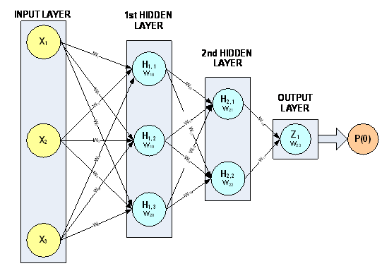
Figure 33, A 3-layer, Feed Forward Network with 3 Input Attributes and 6 Perceptrons
This network has a total of 23 weights. The first nine weights, labeled W1, W2, …, W9, are the weights assigned to the links connecting the network inputs to the perceptrons in the first hidden layer. Note that W1, W2, W4, W5, W7, and W8 are assigned to the two nominal attributes and W3, W6 and W9 are assigned to the continuous attribute. All neural network functions in the C Stat Library use this weight ordering. Weights for all nominal attributes are placed before the weights for any continuous attributes.
PERCEPTRON | POTENTIAL |
|---|---|
H1,1 | |
H1,2 | |
H1,3 | |
H2,1 | |
H2,2 | |
Z1 |
The next six weights are the weights between the first and second hidden layers, and W16 and W17 are the weights for the links connecting the second hidden layer to the output layer. The last six elements in the weights array are the perceptron bias weights. These weights, W18, W19, …, W23 are the weights for perceptrons H1,1, …,H1,3, H2,1…, H2,3, and Z1, respectively.
The perceptron potential calculations for this network are described in the table above. Following the notation presented in the introduction to this chapter, are the perceptron activations from perceptrons H1,1, …,H1,3, H2,1…, H2,3, respectively.
All initialization algorithms in mlff_initialize_weights set the weights for perceptrons not linked directly to the input perceptrons in the same manner. Bias weights for perceptrons not directly linked to input attributes are set to zero. All non-bias weights for these same perceptrons are assigned a value of 1/k where k=the number of links into that perceptron (network->nodes[i].n_inlinks).
For example, in this network, the last three bias weights W21, W22 and W23 are initialized to zero since perceptrons H2,1, H2,1 and Z1 and not directly connected to the input attributes. The other weights to perceptrons H2,1 and H2,2 are assigned a value of one half since these perceptrons each have only two input links. The weights to the output perceptron, Z1, are also one half since Z1 has two inputs links.
The calculation of the weights for the links between the input attributes and their perceptrons are initialized differently by the four algorithms. All algorithms, however, scale these weights so that the average potential for the first layer perceptrons is zero. This reduces the possibility of saturation or numerical overflow during the initial stages of optimization.
Equal Weights (method=IMSLS_EQUAL)
In this algorithm, the non-bias weights for each link between the input attributes and the perceptrons in the first layer are initialized to:
where Wi is the weight for all links between the i-th input attributes, n is equal to the total number of input attributes and Si is equal to the standard deviation of the potential for the i-th input attribute. In the above example, the values for weights W1, W2, …, W9, each would be set to:
since this network has three input attributes.
Next the average potential for each of the perceptrons connected to the input layer is calculated by:
where is equal to the average potential for the i-th input attribute. All other bias weights are set to zero.
Random Weights (method=IMSLS_RANDOM)
This algorithm first generates random values for the input layer weights using the Uniform [-0.5, +0.5] distribution. These are then scaled using the standard deviation of the input layer potentials.
where U is a random number uniformly distributed on the interval [-0.5,+0.5] and Si is equal to the standard deviation of the potential for the i-th input attribute.
Next the average potential for each of the perceptrons connected to the input layer is calculated by:
where is equal to the average potential for the i-th input attribute. All other bias weights are set to zero.
Principal Component Weights (method=IMSLS_PRINCIPAL_COMPONENTS)
This uses principal component analysis to generate weights. The arrays nominal and continuous are combined into a single matrix. The correlation matrix of this matrix is decomposed using principal component analysis. The elements of the principal components from this analysis are used to initialize weights associated with the network inputs. As with the other methods the principal component weights are scaled by using the standard deviation of the potential for the perceptrons connected to the input layer:
where Wi is the weight for the link between the i-th input attribute and the j-th perceptron, ξij is the i-th value of the j-th principal component, and Si is equal to the standard deviation of the potential for the i-th input attribute.
If the number of principal components is less than the number of perceptrons in the first layer, i.e., (n_continuous+n_nominal) < n_layer1, where n_layer1 is the number of perceptrons in the first layer, then it is not possible to initialize all weights with principal components. In this case, the first (n_continuous + n_nominal) perceptrons are initialized using the principal components and then the remainder are initialized using random weights (method=IMSLS_RANDOM).
As with the other methods, the bias weights for each of the first layer perceptrons is set to ensure that the average potential in this layer is equal to zero:
where is equal to the average potential for the link between i-th input attribute and the j-th first layer perceptron, and is the standard deviation for this same potential.
Discriminant Weights (method=IMSLS_DISCRIMINANT)
This method is very similar to principal component weights. Instead the discriminant analysis elements replace the principal component elements. The weights between the i-th input attribute and the j-th perceptron in the first layer are calculated by:
Where Wi is the weight for the link between the i-th input attribute and the j-th perceptron, θij is the i-th value of the j-th discriminant component, and Si is equal to the standard deviation of the potential for the i-th input attribute.
If the number of discriminant components is less than the number of perceptrons in the first layer, i.e., (n_continuous + n_nominal) < n_layer1, where n_layer1 is the number of perceptrons in the first layer, then it is not possible to initialize all weights with components from the discriminant analysis. In this case, the first (n_continuous + n_nominal) perceptrons are initialized using the discriminant components and then the remainder are initialized using random weights (method=IMSLS_RANDOM).
As with the other methods, the bias weights for each of the first layer perceptrons is set to ensure that the average potential in this layer is equal to zero:
where is equal to the average potential for the link between i-th input attribute and the j-th first layer perceptron, and Sij is the standard deviation for this same potential.
Examples
Example 1
This example illustrates random initialization algorithms for a three layer network with one output. The first and second hidden layers contain three and two perceptrons for a total of five network perceptrons, respectively.
The nine input attributes consist of two continuous attributes plus seven binary attributes encoded from two nominal attributes using binary encoding.
The weights are initialized using the random weights algorithm. This results in different weights for every perceptron in the first hidden layer. The weights in other layers are initialized using equal weights. It should be noted that the bias weights in the first layer are not random. Except for the discriminant weights algorithm, the bias weights are always calculated to ensure that the average potential for each perceptron in the first layer is zero.
#include <stdio.h>
#include <imsls.h>
int main(){
Imsls_f_NN_Network *network;
int i, j, k, m;
int n_patterns =24; /* no. of training patterns */
int n_nvars =2; /* 2 nominal unencoded variables */
int n_nominal =7; /* 7 inputs for the binary encoded
nominal vars */
int n_continuous =2; /* 2 continuous input attributes */
int nominalIn[24]; /* work arrays used to encode */
int *nominalOut; /* nominal data */
int n_classes;
int classification[24] = {
0, 0, 0, 0, 0, 0, 1, 1, 1, 1, 1, 1,
0, 0, 0, 0, 0, 0, 1, 1, 1, 1, 1, 1
};
/* raw nominal input data */
int nominal_unencododed[2*24] =
{
0, 0, 0, 1, 0, 2,
1, 0, 1, 1, 1, 2,
2, 0, 2, 1, 2, 2,
3, 0, 3, 1, 3, 2,
0, 0, 0, 1, 0, 2,
1, 0, 1, 1, 1, 2,
2, 0, 2, 1, 2, 2,
3, 0, 3, 1, 3, 2
};
/* input array for binary encoded version of
nominal_unencododed[] array above */
int nominal[7*24];
float *weights;
float continuous[2*24] =
{
0.00,0.00,0.02,0.02,0.04,0.04,0.06,0.06,0.08,0.08,0.10,0.10,
0.12,0.12,0.14,0.14,0.16,0.16,0.18,0.18,0.20,0.20,0.22,0.22,
0.24,0.28,0.26,0.30,0.28,0.32,0.30,0.34,0.32,0.36,0.34,0.38,
0.36,0.40,0.38,0.42,0.40,0.44,0.42,0.46,0.44,0.48,0.46,0.50
};
/* Setup Nominal Input Attributes Using Binary Encoding */
m=0;
for (i=0; i<n_nvars; i++){
for (j=0; j<n_patterns; j++) {
nominalIn[j] = nominal_unencododed[2*j+i] + 1;
}
nominalOut = imsls_unsupervised_nominal_filter(n_patterns,
&n_classes, nominalIn, 0);
for(k=0; k<n_classes; k++){
for(j=0; j<n_patterns; j++){
nominal[j*n_nominal+m] = nominalOut[j*n_classes+k];
}
m++;
}
}
printf("\tINPUT TRAINING PATTERNS\n");
printf("\tY Nom1 Nom2 X0 X1 \n");
for(i=0; i<n_patterns; i++){
printf("\t%d %d \t %d %f %f \n", classification[i],
nominal_unencododed[i*2], nominal_unencododed[i*2+1],
continuous[i*2], continuous[i*2+1]);
}
/* Binary classification network 9 inputs 1 output = 2 classes */
network = imsls_f_mlff_network_init(9, 1);
imsls_f_mlff_network(network, IMSLS_CREATE_HIDDEN_LAYER, 3, 0);
imsls_f_mlff_network(network, IMSLS_CREATE_HIDDEN_LAYER, 2,
IMSLS_LINK_ALL, 0);
/* Note the following statement is for repeatable output */
imsls_random_seed_set(5555);
/* Random Weights */
weights = imsls_f_mlff_initialize_weights(network, n_patterns,
n_nominal, n_continuous, nominal, continuous,
IMSLS_PRINT, 0);
}
Output
INPUT TRAINING PATTERNS
Y Nom1 Nom2 X0 X1
0 0 0 0.000000 0.000000
0 0 1 0.020000 0.020000
0 0 2 0.040000 0.040000
0 1 0 0.060000 0.060000
0 1 1 0.080000 0.080000
0 1 2 0.100000 0.100000
1 2 0 0.120000 0.120000
1 2 1 0.140000 0.140000
1 2 2 0.160000 0.160000
1 3 0 0.180000 0.180000
1 3 1 0.200000 0.200000
1 3 2 0.220000 0.220000
0 0 0 0.240000 0.280000
0 0 1 0.260000 0.300000
0 0 2 0.280000 0.320000
0 1 0 0.300000 0.340000
0 1 1 0.320000 0.360000
0 1 2 0.340000 0.380000
1 2 0 0.360000 0.400000
1 2 1 0.380000 0.420000
1 2 2 0.400000 0.440000
1 3 0 0.420000 0.460000
1 3 1 0.440000 0.480000
1 3 2 0.460000 0.500000
-------------------------------------------
- NETWORK WEIGHTS INITIALIZED USING
- RANDOM WEIGHTS
- Input Attributes: 9
- Nominal: 2
- Nominal(encoded): 7
- Continuous: 2
- Output Attributes: 1
- Layers: 3
- Perceptrons: 6
- Weights: 41
- Patterns: 24
-------------------------------------------
------------- HIDDEN LAYER 1 -------------
--- Perceptron 0 ---
Link from Input Node Weight
N0 0.937069
N1 -0.547569
N2 1.468248
N3 0.107160
N4 -0.884992
N5 -0.814069
N6 -1.979680
X7 -0.041228
X8 -1.368315
Bias 3.3099
--- Perceptron 1 ---
Link from Input Node Weight
N0 -0.308421
N1 -1.058450
N2 -0.981207
N3 1.040820
N4 -0.033493
N5 -0.575732
N6 0.571939
X7 0.811886
X8 -0.415498
Bias 0.573286
--- Perceptron 2 ---
Link from Input Node Weight
N0 -1.117744
N1 0.620799
N2 0.174895
N3 -0.100458
N4 -0.961071
N5 0.854179
N6 0.046423
X7 0.880998
X8 -0.903982
Bias 1.00437
-------------------------------------------
------------- HIDDEN LAYER 2 -------------
--- Perceptron 0 ---
Link from Input Node Weight
P0 0.333333
P1 0.333333
P2 0.333333
Bias 0
--- Perceptron 1 ---
Link from Input Node Weight
P0 0.333333
P1 0.333333
P2 0.333333
Bias 0
-------------------------------------------
------------- OUTPUT LAYER -------------
--- Perceptron 0 ---
Link from Input Node Weight
P3 0.500000
P4 0.500000
Bias 0
-------------------------------------------
Example 2
This example illustrates the discriminant weights initialization algorithm for a three layer network with one output. The first and second hidden layers contain three and two perceptrons for a total of five network perceptrons, respectively.
The data are the same as Example 1, and the network structure is the same except that all nominal input attributes are removed. This was necessary since the discriminant weights algorithm only works when all input attributes are continuous.
The discriminant weights algorithm initializes the weights in the first hidden layer to the coefficients of the discriminant functions. Since this example is a binary classification example, the number of discriminant functions is equal to the number of classes, two, but there are three perceptrons in the first layer. The weights for the first two perceptrons in this layer are the discriminant function coefficients, including the bias weight. The weights for the last perceptron in this layer were determined randomly.
#include <stdio.h>
#include <imsls.h>
int main(){
Imsls_f_NN_Network *network;
int i, j, k, m;
int n_patterns =24; /* no. of training patterns */
int n_continuous =2; /* 2 continuous input attributes */
int classification[24] = {
0, 0, 0, 0, 0, 0, 1, 1, 1, 1, 1, 1,
0, 0, 0, 0, 0, 0, 1, 1, 1, 1, 1, 1
};
float *weights;
float continuous[2*24] =
{
0.00,0.00,0.02,0.02,0.04,0.04,0.06,0.06,0.08,0.08,0.10,0.10,
0.12,0.12,0.14,0.14,0.16,0.16,0.18,0.18,0.20,0.20,0.22,0.22,
0.24,0.28,0.26,0.30,0.28,0.32,0.30,0.34,0.32,0.36,0.34,0.38,
0.36,0.40,0.38,0.42,0.40,0.44,0.42,0.46,0.44,0.48,0.46,0.50
};
printf("\tINPUT TRAINING PATTERNS\n");
printf("\tY X0 X1 \n");
for(i=0; i<n_patterns; i++){
printf("\t%d %f %f \n", classification[i],
continuous[i*2], continuous[i*2+1]);
}
/* Binary classification network 2 inputs 1 output = 2 classes */
network = imsls_f_mlff_network_init(2, 1);
imsls_f_mlff_network(network, IMSLS_CREATE_HIDDEN_LAYER, 3, 0);
imsls_f_mlff_network(network, IMSLS_CREATE_HIDDEN_LAYER, 2,
IMSLS_LINK_ALL, 0);
/* Discriminant weights */
/* Set seed for consistent results */
imsls_random_seed_set(12357);
weights = imsls_f_mlff_initialize_weights(network, n_patterns,
0, n_continuous, NULL, continuous,
IMSLS_METHOD, IMSLS_DISCRIMINANT,
IMSLS_CLASSIFICATION, classification,
IMSLS_PRINT, 0);
}
Output
INPUT TRAINING PATTERNS
Y X0 X1
0 0.000000 0.000000
0 0.020000 0.020000
0 0.040000 0.040000
0 0.060000 0.060000
0 0.080000 0.080000
0 0.100000 0.100000
1 0.120000 0.120000
1 0.140000 0.140000
1 0.160000 0.160000
1 0.180000 0.180000
1 0.200000 0.200000
1 0.220000 0.220000
0 0.240000 0.280000
0 0.260000 0.300000
0 0.280000 0.320000
0 0.300000 0.340000
0 0.320000 0.360000
0 0.340000 0.380000
1 0.360000 0.400000
1 0.380000 0.420000
1 0.400000 0.440000
1 0.420000 0.460000
1 0.440000 0.480000
1 0.460000 0.500000
Discriminant Analysis Classification Error Rate = 0.000000
-------------------------------------------
- NETWORK WEIGHTS INITIALIZED USING
- DISCRIMINANT WEIGHTS
- Input Attributes: 2
- Nominal: 0
- Nominal(encoded): 0
- Continuous: 2
- Output Attributes: 1
- n_classes: 2
- Layers: 3
- Perceptrons: 6
- Weights: 20
- Patterns: 24
-------------------------------------------
------------- HIDDEN LAYER 1 -------------
--- Perceptron 0 ---
Link from Input Node Weight
X0 229.165253
X1 -189.879715
Bias -2.13362
--- Perceptron 1 ---
Link from Input Node Weight
X0 889.167236
X1 -755.595703
Bias -12.5051
--- Perceptron 2 ---
Link from Input Node Weight
X0 -4.495886
X1 -0.976032
Bias 6.07217
-------------------------------------------
------------- HIDDEN LAYER 2 -------------
--- Perceptron 0 ---
Link from Input Node Weight
P0 0.333333
P1 0.333333
P2 0.333333
Bias 0
--- Perceptron 1 ---
Link from Input Node Weight
P0 0.333333
P1 0.333333
P2 0.333333
Bias 0
-------------------------------------------
------------- OUTPUT LAYER -------------
--- Perceptron 0 ---
Link from Input Node Weight
P3 0.500000
P4 0.500000
Bias 0
-------------------------------------------


