RCURV
Fits a polynomial curve using least squares.
Required Arguments
XDATA — Vector of length NOBS containing the x values. (Input)
YDATA — Vector of length NOBS containing the y values. (Input)
B — Vector of length NDEG + 1 containing the coefficients . (Output)
The fitted polynomial is
Optional Arguments
NOBS — Number of observations. (Input)
Default: NOBS = size (XDATA,1).
Default: NOBS = size (XDATA,1).
NDEG — Degree of polynomial. (Input)
Default: NDEG = size (B,1) - 1.
Default: NDEG = size (B,1) - 1.
SSPOLY — Vector of length NDEG + 1 containing the sequential sums of squares. (Output)
SSPOLY(1) contains the sum of squares due to the mean. For i = 1, 2, …, NDEG, SSPOLY(i + 1) contains the sum of squares due to xi adjusted for the mean, x, x2, …, and xi-1.
SSPOLY(1) contains the sum of squares due to the mean. For i = 1, 2, …, NDEG, SSPOLY(i + 1) contains the sum of squares due to xi adjusted for the mean, x, x2, …, and xi-1.
STAT — Vector of length 10 containing statistics described below. (Output)
i | Statistics |
|---|---|
1 | Mean of x |
2 | Mean of y |
3 | Sample variance of x |
4 | Sample variance of y |
5 | R-squared (in percent) |
6 | Degrees of freedom for regression |
7 | Regression sum of squares |
8 | Degrees of freedom for error |
9 | Error sum of squares |
10 | Number of data points (x, y) containing NaN (not a number) as a x or y value |
FORTRAN 90 Interface
Generic: CALL RCURV (XDATA, YDATA, B [, …])
Specific: The specific interface names are S_RCURV and D_RCURV.
FORTRAN 77 Interface
Single: CALL RCURV (NOBS, XDATA, YDATA, NDEG, B, SSPOLY, STAT)
Double: The double precision name is DRCURV.
Description
Routine RCURV computes estimates of the regression coefficients in a polynomial (curvilinear) regression model. In addition to the computation of the fit, RCURV computes some summary statistics. Sequential sums of squares attributable to each power of the independent variable (stored in SSPOLY) are computed. These are useful in assessing the importance of the higher order powers in the fit. Draper and Smith (1981, pages 101− 102) and Neter and Wasserman (1974, pages 278−287) discuss the interpretation of the sequential sums of squares. The statistic R2 (stored in STAT(5)) is the percentage of the sum of squares of y about its mean explained by the polynomial curve. Specifically,
where
is the fitted y value at xi and
(stored in STAT(2)) is the mean of y. This statistic is useful in assessing the overall fit of the curve to the data. R2 must be between 0% and 100%, inclusive. R2 = 100% indicates a perfect fit to the data.
Routine RCURV computes estimates of the regression coefficients in a polynomial model using orthogonal polynomials as the regressor variables. This reparameterization of the polynomial model in terms of orthogonal polynomials has the advantage that the loss of accuracy resulting from forming powers of the x-values is avoided. All results are returned to the user for the original model.
The routine RCURV is based on the algorithm of Forsythe (1957). A modification to Forsythe’s algorithm suggested by Shampine (1975) is used for computing the polynomial coefficients. A discussion of Forsythe’s algorithm and Shampine’s modification appears in Kennedy and Gentle (1980, pages 342−347).
Comments
1. Workspace may be explicitly provided, if desired, by use of R2URV/DR2URV. The reference is:
CALL R2URV (NOBS, XDATA, YDATA, NDEG, B, SSPOLY, STAT, WK, IWK)
The additional arguments are as follows:
WK — Work vector of length 11 * NOBS + 11 * NDEG + 5 + (NDEG + 1) * (NDEG + 3).
IWK — Work vector of length NOBS.
2. Informational errors
Type | Code | Description |
|---|---|---|
4 | 3 | Each (x, y) point contains NaN (not a number). There are no valid data. |
4 | 7 | The x values are constant. At least NDEG + 1 distinct x values are needed to fit a NDEG polynomial. |
3 | 4 | The y values are constant. A zero order polynomial is fit. High order coefficients are set to zero. |
3 | 5 | There are too few observations to fit the desired degree polynomial. High order coefficients are set to zero. |
3 | 6 | A perfect fit was obtained with a polynomial of degree less than NDEG. High order coefficients are set to zero. |
3. If NDEG is greater than 10, the accuracy of the results may be questionable.
Example
A polynomial model is fitted to data discussed by Neter and Wasserman (1974, pages 279− 285). The data set contains the response variable y measuring coffee sales (in hundred gallons) and the number of self-service coffee dispensers. Responses for fourteen similar cafeterias are in the data set.
USE RCURV_INT
USE WRRRL_INT
USE WRRRN_INT
IMPLICIT NONE
INTEGER NDEG, NOBS
PARAMETER (NDEG=2, NOBS=14)
!
REAL B(NDEG+1), SSPOLY(NDEG+1), STAT(10), XDATA(NOBS),&
YDATA(NOBS)
CHARACTER CLABEL(11)*15, RLABEL(1)*4
!
DATA RLABEL/'NONE'/, CLABEL/' ', 'Mean of X', 'Mean of Y',&
'Variance X', 'Variance Y', 'R-squared',&
'DF Reg.', 'SS Reg.', 'DF Error', 'SS Error',&
'Pts. with NaN'/
DATA XDATA/0., 0., 1., 1., 2., 2., 4., 4., 5., 5., 6., 6., 7.,&
7./
DATA YDATA/508.1, 498.4, 568.2, 577.3, 651.7, 657.0, 755.3,&
758.9, 787.6, 792.1, 841.4, 831.8, 854.7, 871.4/
!
CALL RCURV (XDATA, YDATA, B, SSPOLY=SSPOLY, STAT=STAT)
!
CALL WRRRN ('B', B, 1, NDEG+1, 1)
CALL WRRRN ('SSPOLY', SSPOLY, 1, NDEG+1, 1)
CALL WRRRL ('%/STAT', STAT, RLABEL, CLABEL, 1, 10, 1, &
FMT='(2W10.4)')
END
Output
B
1 2 3
503.3 78.9 -4.0
SSPOLY
1 2 3
7077152.0 220644.2 4387.7
STAT
Mean of X Mean of Y Variance X Variance Y R-squared DF Reg.
3.571 711.0 6.418 17364.8 99.69 2
SS Reg. DF Error SS Error Pts. with NaN
225031.9 11 710.5 0
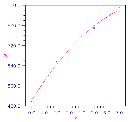
Figure 8, Plot of Data and Second Degree Polynomial Fit


