BSVLS
Computes the variable knot B-spline least squares approximation to given data.
Required Arguments
XDATA — Array of length NDATA containing the data point abscissas. (Input)
FDATA — Array of length NDATA containing the data point ordinates. (Input)
KORDER — Order of the spline. (Input)
KORDER must be less than or equal to NDATA.
KORDER must be less than or equal to NDATA.
NCOEF — Number of B-spline coefficients. (Input)
NCOEF must be less than or equal to NDATA.
NCOEF must be less than or equal to NDATA.
XGUESS — Array of length NCOEF + KORDER containing the initial guess of knots. (Input)
XGUESS must be nondecreasing.
XGUESS must be nondecreasing.
XKNOT — Array of length NCOEF + KORDER containing the (nondecreasing) knot sequence. (Output)
BSCOEF — Array of length NCOEF containing the B-spline representation. (Output)
SSQ — The square root of the sum of the squares of the error. (Output)
Optional Arguments
NDATA — Number of data points. (Input)
NDATA must be at least 2.
Default: NDATA = size(XDATA, 1)
NDATA must be at least 2.
Default: NDATA = size(XDATA, 1)
WEIGHT — Array of length NDATA containing the weights. (Input)
Default: WEIGHT = 1.0.
Default: WEIGHT = 1.0.
FORTRAN 90 Interface
Generic: CALL BSVLS (XDATA, FDATA, KORDER, NCOEF, XGUESS, XKNOT, BSCOEF,
SSQ [, …])
SSQ [, …])
Specific: The specific interface names are S_BSVLS and D_BSVLS.
FORTRAN 77 Interface
Single: CALL BSVLS (NDATA, XDATA, FDATA, WEIGHT, KORDER, NCOEF, XGUESS, XKNOT, BSCOEF, SSQ)
Double: The double precision name is DBSVLS.
Description
The routine BSVLS attempts to find the best placement of knots that will minimize the leastsquares error to given data by a spline of order k = KORDER with N = NCOEF coefficients. The user provides the order k of the spline and the number of coefficients N. For this problem to make sense, it is necessary that N > k. We then attempt to find the minimum of the functional
The user must provide the weights w = WEIGHT, the data xi = XDATA and fi = FDATA, and
M = NDATA. The minimum is taken over all admissible knot sequences t.
M = NDATA. The minimum is taken over all admissible knot sequences t.
The technique employed in BSVLS uses the fact that for a fixed knot sequence t the minimization in a is a linear least-squares problem that can be solved by calling the IMSL routine BSLSQ. Thus, we can think of our objective function F as a function of just t by setting
A Gauss-Seidel (cyclic coordinate) method is then used to reduce the value of the new objective function G. In addition to this local method, there is a global heuristic built into the algorithm that will be useful if the data arise from a smooth function. This heuristic is based on the routine NEWNOT of de Boor (1978, pages 184 and 258− 261).
The user must input an initial guess, tg = XGUESS, for the knot sequence. This guess must be a valid knot sequence for the splines of order k with
with tg nondecreasing, and
The routine BSVLS returns the B-spline representation of the best fit found by the algorithm as well as the square root of the sum of squares error in SSQ. If this answer is unsatisfactory, you may reinitialize BSVLS with the return from BSVLS to see if an improvement will occur. We have found that this option does not usually (substantially) improve the result. In regard to execution speed, this routine can be several orders of magnitude slower than one call to the least-squares routine BSLSQ.
Comments
1. Workspace may be explicitly provided, if desired, by use of B2VLS/DB2VLS. The reference is:
CALL B2VLS (NDATA, XDATA, FDATA, WEIGHT, KORDER, NCOEF, XGUESS, XKNOT, BSCOEF, SSQ, IWK, WK)
The additional arguments are as follows:
IWK — Work array of length NDATA.
WK — Work array of length NCOEF * (6 + 2 * KORDER) + KORDER * (7 − KORDER) +
3 * NDATA + 3.
3 * NDATA + 3.
2. Informational errors
Type | Code | Description |
|---|---|---|
3 | 12 | The knots found to be optimal are stacked more than KORDER. This indicates fewer knots will produce the same error sum of squares. The knots have been separated slightly. |
4 | 9 | The multiplicity of the knots in XGUESS cannot exceed the order of the spline. |
4 | 10 | XGUESS must be nondecreasing. |
Example
In this example, we try to fit the function ∣x − .33∣ evaluated at 100 equally spaced points on [0, 1]. We first use quadratic splines with 2 interior knots initially at .2 and .8. The eventual error should be zero since the function is a quadratic spline with two knots stacked at .33. As a second example, we try to fit the same data with cubic splines with three interior knots initially located at .1, .2, and, .5. Again, the theoretical error is zero when the three knots are stacked at .33.
We include a graph of the initial least-squares fit using the IMSL routine BSLSQ for the above quadratic spline example with knots at .2 and .8. This graph overlays the graph of the spline computed by BSVLS, which is indistinguishable from the data.
USE BSVLS_INT
USE UMACH_INT
IMPLICIT NONE
INTEGER KORD1, KORD2, NCOEF1, NCOEF2, NDATA
PARAMETER (KORD1=3, KORD2=4, NCOEF1=5, NCOEF2=7, NDATA=100)
!
INTEGER I, NOUT
REAL ABS, BSCOEF(NCOEF2), F, FDATA(NDATA), FLOAT, SSQ,&
WEIGHT(NDATA), X, XDATA(NDATA), XGUES1(NCOEF1+KORD1),&
XGUES2(KORD2+NCOEF2), XKNOT(NCOEF2+KORD2)
INTRINSIC ABS, FLOAT
!
DATA XGUES1/3*0.0, .2, .8, 3*1.0001/
DATA XGUES2/4*0.0, .1, .2, .5, 4*1.0001/
DATA WEIGHT/NDATA*.01/
! Define function
F(X) = ABS(X-.33)
! Set up data
DO 10 I=1, NDATA
XDATA(I) = FLOAT(I-1)/FLOAT(NDATA)
FDATA(I) = F(XDATA(I))
10 CONTINUE
! Compute least squares B-spline
! representation with KORD1, NCOEF1,
! and XGUES1.
CALL BSVLS (XDATA, FDATA, KORD1, NCOEF1, XGUES1,&
XKNOT, BSCOEF, SSQ, WEIGHT=WEIGHT)
! Get output unit number
CALL UMACH (2, NOUT)
! Print heading
WRITE (NOUT,99998) 'quadratic'
! Print SSQ and the knots
WRITE (NOUT,99999) SSQ, (XKNOT(I),I=1,KORD1+NCOEF1)
! Compute least squares B-spline
! representation with KORD2, NCOEF2,
! and XGUES2.
CALL BSVLS (XDATA, FDATA, KORD2, NCOEF2, XGUES2,&
XKNOT, BSCOEF, SSQ, WEIGHT=WEIGHT)
! Print SSQ and the knots
WRITE (NOUT,99998) 'cubic'
WRITE (NOUT,99999) SSQ, (XKNOT(I),I=1,KORD2+NCOEF2)
!
99998 FORMAT (' Piecewise ', A, /)
99999 FORMAT (' Square root of the sum of squares : ', F9.4, /,&
' Knot sequence : ', /, 1X, 11(F9.4,/,1X))
END
Output
Piecewise quadratic
Square root of the sum of squares : 0.0008
Knot sequence :
0.0000
0.0000
0.0000
0.3137
0.3464
1.0001
1.0001
1.0001
Piecewise cubic
Square root of the sum of squares : 0.0005
Knot sequence :
0.0000
0.0000
0.0000
0.0000
0.3167
0.3273
0.3464
1.0001
1.0001
1.0001
1.0001
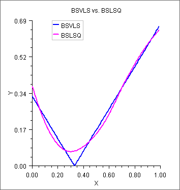
Figure 9, BSVLS vs. BSLSQ


