CONFT

Computes the least-squares constrained spline approximation, returning the B-spline coefficients.
Required Arguments
XDATA — Array of length NDATA containing the data point abscissas. (Input)
FDATA — Array of size NDATA containing the values to be approximated. (Input)
FDATA(I) contains the value at XDATA(I).
FDATA(I) contains the value at XDATA(I).
XVAL — Array of length NXVAL containing the abscissas at which the fit is to be constrained. (Input)
NHARD — Number of entries of XVAL involved in the ‘hard’ constraints. (Input)
Note: (0 ≤ NHARD ≤ NXVAL). Setting NHARD to zero always results in a fit, while setting NHARD to NXVAL forces all constraints to be met. The ‘hard’ constraints must be satisfied or else the routine signals failure. The ‘soft’ constraints need not be satisfied, but there will be an attempt to satisfy the ‘soft’ constraints. The constraints must be ordered in terms of priority with the most important constraints first. Thus, all of the ‘hard’ constraints must preceed the ‘soft’ constraints. If infeasibility is detected among the soft constraints, we satisfy (in order) as many of the soft constraints as possible.
Note: (0 ≤ NHARD ≤ NXVAL). Setting NHARD to zero always results in a fit, while setting NHARD to NXVAL forces all constraints to be met. The ‘hard’ constraints must be satisfied or else the routine signals failure. The ‘soft’ constraints need not be satisfied, but there will be an attempt to satisfy the ‘soft’ constraints. The constraints must be ordered in terms of priority with the most important constraints first. Thus, all of the ‘hard’ constraints must preceed the ‘soft’ constraints. If infeasibility is detected among the soft constraints, we satisfy (in order) as many of the soft constraints as possible.
IDER — Array of length NXVAL containing the derivative value of the spline that is to be constrained. (Input)
If we want to constrain the integral of the spline over the closed interval (c, d), then we set IDER(I) = IDER(I + 1) = − 1 and XVAL(I) = c and XVAL(I + 1) = d. For consistency, we insist that ITYPE(I) = ITYPE(I + 1) .GE. 0 and c .LE. d. Note that every entry in IDER must be at least − 1.
If we want to constrain the integral of the spline over the closed interval (c, d), then we set IDER(I) = IDER(I + 1) = − 1 and XVAL(I) = c and XVAL(I + 1) = d. For consistency, we insist that ITYPE(I) = ITYPE(I + 1) .GE. 0 and c .LE. d. Note that every entry in IDER must be at least − 1.
ITYPE — Array of length NXVAL indicating the types of general constraints. (Input)
ITYPE(I) | I-th Constraint |
|---|---|
1 | |
2 | |
3 | |
4 | |
(di = ‑1)1 | |
(di = ‑1)2 | |
(di = ‑1)3 | |
(di = ‑1)4 | |
10 | periodic end conditions |
99 | disregard this constraint |
In order to set two point constraints, we must have ITYPE(I) = ITYPE(I + 1) and ITYPE(I) must be negative.
ITYPE(I) | I-th Constraint |
|---|---|
‑1 | |
‑2 | |
‑3 | |
‑4 |
BL — Array of length NXVAL containing the lower limit of the general constraints, if there is no lower limit on the I-th constraint, then BL(I) is not referenced. (Input)
BU — Array of length NXVAL containing the upper limit of the general constraints, if there is no upper limit on the I-th constraint, then BU(I) is not referenced; if there is no range constraint, BL and BU can share the same storage locations. (Input)
If the I-th constraint is an equality constraint, BU(I) is not referenced.
If the I-th constraint is an equality constraint, BU(I) is not referenced.
KORDER — Order of the spline. (Input)
XKNOT — Array of length NCOEF + KORDER containing the knot sequence. (Input)
The entries of XKNOT must be nondecreasing.
The entries of XKNOT must be nondecreasing.
BSCOEF — Array of length NCOEF containing the B-spline coefficients. (Output)
Optional Arguments
NDATA — Number of data points. (Input)
Default: NDATA = size (XDATA,1).
Default: NDATA = size (XDATA,1).
WEIGHT — Array of length NDATA containing the weights. (Input)
Default: WEIGHT = 1.0.
Default: WEIGHT = 1.0.
NXVAL — Number of points in the vector XVAL. (Input)
Default: NXVAL = size (XVAL,1).
Default: NXVAL = size (XVAL,1).
NCOEF — Number of B-spline coefficients. (Input)
Default: NCOEF = size (BSCOEF,1).
Default: NCOEF = size (BSCOEF,1).
FORTRAN 90 Interface
Generic: CALL CONFT (XDATA, FDATA, XVAL, NHARD, IDER, ITYPE, BL, BU, KORDER, XKNOT, BSCOEF [, …])
Specific: The specific interface names are S_CONFT and D_CONFT.
FORTRAN 77 Interface
Single: CALL CONFT (NDATA, XDATA, FDATA, WEIGHT, NXVAL, XVAL, NHARD, IDER, ITYPE, BL, BU, KORDER, XKNOT, NCOEF, BSCOEF)
Double: The double precision name is DCONFT.
Description
The routine CONFT produces a constrained, weighted least-squares fit to data from a spline subspace. Constraints involving one point, two points, or integrals over an interval are allowed. The types of constraints supported by the routine are of four types.
An interval, Ip, (which may be a point, a finite interval , or semi-infinite interval) is associated with each of these constraints.
The input for this routine consists of several items, first, the data set (xi, fi) for i = 1, …, N (where N = NDATA), that is the data which is to be fit. Second, we have the weights to be used in the least squares fit (w = WEIGHT). The vector XVAL of length NXVAL contains the abscissas of the points involved in specifying the constraints. The algorithm tries to satisfy all the constraints, but if the constraints are inconsistent then it will drop constraints, in the reverse order specified, until either a consistent set of constraints is found or the “hard” constraints are determined to be inconsistent (the “hard” constraints are those involving XVAL(1), …, XVAL(NHARD)). Thus, the algorithm satisfies as many constraints as possible in the order specified by the user. In the case when constraints are dropped, the user will receive a message explaining how many constraints had to be dropped to obtain the fit. The next several arguments are related to the type of constraint and the constraint interval. The last four arguments determine the spline solution. The user chooses the spline subspace (KORDER, XKNOT, and NCOEF), and the routine returns the B-spline coefficients in BSCOEF.
Let nf denote the number of feasible constraints as described above. Then, the routine solves the problem.
This linearly constrained least-squares problem is treated as a quadratic program and is solved by invoking the IMSL routine QPROG (see Chapter 8, “Optimization”).
The choice of weights depends on the data uncertainty in the problem. In some cases, there is a natural choice for the weights based on the estimates of errors in the data points.
Determining feasibility of linear constraints is a numerically sensitive task. If you encounter difficulties, a quick fix would be to widen the constraint intervals Ip.
Comments
1. Workspace may be explicitly provided, if desired, by use of C2NFT/DC2NFT. The reference is:
CALL C2NFT (NDATA, XDATA, FDATA, WEIGHT, NXVAL, XVAL, NHARD, IDER, ITYPE, BL, BU, KORDER, XKNOT, NCOEF, BSCOEF, H, G, A, RHS, WK, IPERM, IWK)
The additional arguments are as follows:
H — Work array of size NCOEF by NCOEF. Upon output, H contains the Hessian matrix of the objective function used in the call to QPROG (see Chapter 8, “Optimization”).
G — Work array of size NCOEF. Upon output, G contains the coefficients of the linear term used in the call to QPROG.
A — Work array of size (2 * NXVAL + KORDER) by (NCOEF + 1). Upon output, A contains the constraint matrix used in the call QPROG. The last column of A is used to keep record of the original order of the constraints.
RHS — Work array of size 2 * NXVAL + KORDER . Upon output, RHS contains the right hand side of the constraint matrix A used in the call to QPROG.
WK — Work array of size (KORDER + 1) * (2 * KORDER + 1) + (3 * NCOEF * NCOEF + 13 * NCOEF)/2 + (2 * NXVAL + KORDER +30)*(2*NXVAL + KORDER) + NDATA + 1.
IPERM — Work array of size NXVAL. Upon output, IPERM contains the permutation of the original constraints used to generate the matrix A.
IWK — Work array of size NDATA + 30 * (2 * NXVAL + KORDER) + 4 * NCOEF.
2. Informational errors
Type | Code | Description |
|---|---|---|
3 | 11 | Soft constraints had to be removed in order to get a fit. |
4 | 12 | Multiplicity of the knots cannot exceed the order of the spline. |
4 | 13 | The knots must be nondecreasing. |
4 | 14 | The smallest element of the data point array must be greater than or equal to the KORD-th knot. |
4 | 15 | The largest element of the data point array must be less than or equal to the (NCOEF + 1)st knot. |
4 | 16 | All weights must be greater than zero. |
4 | 17 | The hard constraints could not be met. |
4 | 18 | The abscissas of the constrained points must lie within knot interval. |
4 | 19 | The upperbound must be greater than or equal to the lowerbound for a range constaint. |
4 | 20 | The upper limit of integration must be greater than the lower limit of integration for constraints involving the integral of the approximation. |
Examples
Example 1
This is a simple application of CONFT. We generate data from the function
contaminated with random noise and fit it with cubic splines. The function is increasing so we would hope that our least-squares fit would also be increasing. This is not the case for the unconstrained least squares fit generated by BSLSQ. We then force the derivative to be greater than 0 at NXVAL = 15 equally spaced points and call CONFT. The resulting curve is monotone. We print the error for the two fits averaged over 100 equally spaced points.
USE IMSL_LIBRARIES
IMPLICIT NONE
INTEGER KORDER, NCOEF, NDATA, NXVAL
PARAMETER (KORDER=4, NCOEF=8, NDATA=15, NXVAL=15)
!
INTEGER I, IDER(NXVAL), ITYPE(NXVAL), NHARD, NOUT
REAL ABS, BL(NXVAL), BSCLSQ(NDATA), BSCNFT(NDATA), &
BU(NXVAL), ERRLSQ, ERRNFT, F1, FDATA(NDATA), FLOAT,&
GRDSIZ, SIN, WEIGHT(NDATA), X, XDATA(NDATA),&
XKNOT(KORDER+NDATA), XVAL(NXVAL)
INTRINSIC ABS, FLOAT, SIN
!
F1(X) = .5*X + SIN(.5*X)
! Initialize random number generator
! and get output unit number.
CALL RNSET (234579)
CALL UMACH (2, NOUT)
! Use default weights of one.
!
! Compute original XDATA and FDATA
! with random noise.
GRDSIZ = 10.0
DO 10 I=1, NDATA
XDATA(I) = GRDSIZ*((FLOAT(I-1)/FLOAT(NDATA-1)))
FDATA(I) = RNUNF()
FDATA(I) = F1(XDATA(I)) + (FDATA(I)-.5)
10 CONTINUE
! Compute knots
DO 20 I=1, NCOEF - KORDER + 2
XKNOT(I+KORDER-1) = GRDSIZ*((FLOAT(I-1)/FLOAT(NCOEF-KORDER+1))&
)
20 CONTINUE
DO 30 I=1, KORDER - 1
XKNOT(I) = XKNOT(KORDER)
XKNOT(I+NCOEF+1) = XKNOT(NCOEF+1)
30 CONTINUE
!
! Compute BSLSQ fit.
CALL BSLSQ (XDATA, FDATA, KORDER, XKNOT, NCOEF, BSCLSQ)
! Construct the constraints for
! CONFT.
DO 40 I=1, NXVAL
XVAL(I) = GRDSIZ*FLOAT(I-1)/FLOAT(NXVAL-1)
ITYPE(I) = 3
IDER(I) = 1
BL(I) = 0.0
40 CONTINUE
! Call CONFT
NHARD = 0
CALL CONFT (XDATA, FDATA, XVAL, NHARD, IDER, ITYPE, BL, BU, KORDER,&
XKNOT, BSCNFT, NCOEF=NCOEF)
! Compute the average error
! of 100 points in the interval.
ERRLSQ = 0.0
ERRNFT = 0.0
DO 50 I=1, 100
X = GRDSIZ*FLOAT(I-1)/99.0
ERRNFT = ERRNFT + ABS(F1(X)-BSVAL(X,KORDER,XKNOT,NCOEF,BSCNFT)&
)
ERRLSQ = ERRLSQ + ABS(F1(X)-BSVAL(X,KORDER,XKNOT,NCOEF,BSCLSQ)&
)
50 CONTINUE
! Print results
WRITE (NOUT,99998) ERRLSQ/100.0
WRITE (NOUT,99999) ERRNFT/100.0
!
99998 FORMAT (' Average error with BSLSQ fit: ', F8.5)
99999 FORMAT (' Average error with CONFT fit: ', F8.5)
END
Output
Average error with BSLSQ fit: 0.20250
Average error with CONFT fit: 0.14334
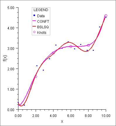
Figure 10, CONFT vs. BSLSQ Forcing Monotonicity
Example 2
We now try to recover the function
from noisy data. We first try the unconstrained least-squares fit using BSLSQ. Finding that fit somewhat unsatisfactory, we apply several constraints using CONFT. First, notice that the unconstrained fit oscillates through the true function at both ends of the interval. This is common for flat data. To remove this oscillation, we constrain the cubic spline to have zero second derivative at the first and last four knots. This forces the cubic spline to reduce to a linear polynomial on the first and last three knot intervals. In addition, we constrain the fit (which we will call s) as follows:
Notice that the last constraint was generated using the periodic option (requiring only the zeroeth derivative to be periodic). We print the error for the two fits averaged over 100 equally spaced points.
USE IMSL_LIBRARIES
IMPLICIT NONE
INTEGER KORDER, NCOEF, NDATA, NXVAL
PARAMETER (KORDER=4, NCOEF=13, NDATA=51, NXVAL=12)
!
INTEGER I, IDER(NXVAL), ITYPE(NXVAL), NHARPT, NOUT
REAL ABS, BL(NXVAL), BSCLSQ(NDATA), BSCNFT(NDATA),&
BU(NXVAL), ERRLSQ, ERRNFT, F1, FDATA(NDATA), FLOAT,&
GRDSIZ, WEIGHT(NDATA), X, XDATA(NDATA),&
XKNOT(KORDER+NDATA), XVAL(NXVAL)
INTRINSIC ABS, FLOAT
!
F1(X) = 1.0/(1.0+X**4)
! Initialize random number generator
! and get output unit number.
CALL UMACH (2, NOUT)
CALL RNSET (234579)
! Use deafult weights of one.
!
! Compute original XDATA and FDATA
! with random noise.
GRDSIZ = 14.0
DO 10 I=1, NDATA
XDATA(I) = GRDSIZ*((FLOAT(I-1)/FLOAT(NDATA-1))) - GRDSIZ/2.0
FDATA(I) = RNUNF()
FDATA(I) = F1(XDATA(I)) + 0.125*(FDATA(I)-.5)
10 CONTINUE
! Compute KNOTS
DO 20 I=1, NCOEF - KORDER + 2
XKNOT(I+KORDER-1) = GRDSIZ*((FLOAT(I-1)/FLOAT(NCOEF-KORDER+1))&
) - GRDSIZ/2.0
20 CONTINUE
DO 30 I=1, KORDER - 1
XKNOT(I) = XKNOT(KORDER)
XKNOT(I+NCOEF+1) = XKNOT(NCOEF+1)
30 CONTINUE
! Compute BSLSQ fit
CALL BSLSQ (XDATA, FDATA, KORDER, XKNOT, NCOEF, BSCLSQ)
! Construct the constraints for
! CONFT
DO 40 I=1, 4
XVAL(I) = XKNOT(KORDER+I-1)
XVAL(I+4) = XKNOT(NCOEF-3+I)
ITYPE(I) = 1
ITYPE(I+4) = 1
IDER(I) = 2
IDER(I+4) = 2
BL(I) = 0.0
BL(I+4) = 0.0
40 CONTINUE
!
XVAL(9) = -7.0
ITYPE(9) = 3
IDER(9) = 0
BL(9) = 0.0
!
XVAL(10) = -7.0
ITYPE(10) = 2
IDER(10) = -1
BU(10) = 2.3
!
XVAL(11) = 7.0
ITYPE(11) = 2
IDER(11) = -1
BU(11) = 2.3
!
XVAL(12) = -7.0
ITYPE(12) = 10
IDER(12) = 0
! Call CONFT
CALL CONFT (XDATA, FDATA, XVAL, NHARPT, IDER, ITYPE, BL, BU,&
KORDER, XKNOT, BSCNFT, NCOEF=NCOEF)
! Compute the average error
! of 100 points in the interval.
ERRLSQ = 0.0
ERRNFT = 0.0
DO 50 I=1, 100
X = GRDSIZ*FLOAT(I-1)/99.0 - GRDSIZ/2.0
ERRNFT = ERRNFT + ABS(F1(X)-BSVAL(X,KORDER,XKNOT,NCOEF,BSCNFT)&
)
ERRLSQ = ERRLSQ + ABS(F1(X)-BSVAL(X,KORDER,XKNOT,NCOEF,BSCLSQ)&
)
50 CONTINUE
! Print results
WRITE (NOUT,99998) ERRLSQ/100.0
WRITE (NOUT,99999) ERRNFT/100.0
!
99998 FORMAT (' Average error with BSLSQ fit: ', F8.5)
99999 FORMAT (' Average error with CONFT fit: ', F8.5)
END
Output
Average error with BSLSQ fit: 0.01783
Average error with CONFT fit: 0.01339
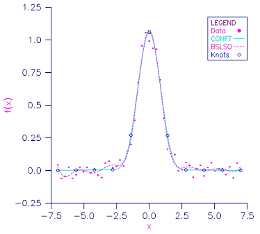
Figure 11, CONFT vs. BSLSQ Approximating 1/(1 + x4)


