RGLM
Fits a multivariate general linear model.
Required Arguments
X — ∣NROW∣ by NCOL matrix containing the data. (Input)
INDCL — Index vector of length NCLVAR containing the column numbers of X that are the classification variables. (Input)
NVEF — Vector of length NEF containing the number of variables associated with each effect in the model. (Input)
INDEF — Index vector of length NVEF(1) + NVEF(2) + … + NVEF(NEF). (Input)
The first NVEF(1) elements give the column numbers of X for each variable in the first effect; the next NVEF(2) elements give the column numbers for each variable in the second effect; and so on. The last NVEF(NEF) elements give the column numbers for each variable in the last effect.
The first NVEF(1) elements give the column numbers of X for each variable in the first effect; the next NVEF(2) elements give the column numbers for each variable in the second effect; and so on. The last NVEF(NEF) elements give the column numbers for each variable in the last effect.
IDEP — Dependent variable option. (Input)
The absolute value of IDEP is the number of dependent (response) variables. The sign of IDEP specifies the following options:
The absolute value of IDEP is the number of dependent (response) variables. The sign of IDEP specifies the following options:
IDEP | Action |
|---|---|
< 0 | The last ‑IDEP columns of X contain the dependent (response) variables. That is, columns NCOL + IDEP + 1, NCOL + IDEP + 2, …, NCOL contain the dependent variables. |
> 0 | The data for the IDEP dependent variables are in the columns of X whose column numbers are given by the elements of INDDEP. |
= 0 | There are no dependent variables. (Generally, this option is not used. However, it is possible to get the R matrix from a QR decomposition of a matrix of regressors in this way.) |
INDDEP — Index vector of length IDEP containing the column numbers of X that are the dependent (response) variables. (Input, if IDEP is positive)
If IDEP is nonpositive, INDDEP is not referenced and can be a vector of length one.
If IDEP is nonpositive, INDDEP is not referenced and can be a vector of length one.
MAXCL — An upper bound on the sum of the number of distinct values taken on by each classification variable. (Input)
B — NCOEF by ∣ IDEP∣ matrix containing on return from the final invocation of this routine a least-squares solution for the regression coefficients. (Output, if IDO = 0 or 1; Input/Output, if IDO = 2 or 3)
Here, NCOEF = IRBEF(NEF + 1) ‑ 1 is the number of coefficients in the model. If INTCEP = 1, row 1 is for the intercept. Column j is for the j-th dependent variable.
Here, NCOEF = IRBEF(NEF + 1) ‑ 1 is the number of coefficients in the model. If INTCEP = 1, row 1 is for the intercept. Column j is for the j-th dependent variable.
IDO | Action |
1 or 2 | A current least-squares solution is given by a solution x to the equation R * x = B |
0 or 3 | A least-squares solution for the regression coefficients is returned in B. Elements of the appropriate row(s) of B are set to 0.0 if linear dependence of the regressors is declared. |
Optional Arguments
IDO — Processing option. (Input)
Default: IDO = 0.
Default: IDO = 0.
IDO | Action |
|---|---|
0 | This is the only invocation of RGLM for this data set, and all the data are input at once. |
1 | This is the first invocation, and additional calls to RGLM will be made. Initialization and updating for the data in X are performed. |
2 | This is an intermediate invocation of RGLM, and updating for the data in X is performed. |
3 | This is the final invocation of this routine. Updating for the data in X and wrap-up computation are performed. |
NROW — The absolute value of NROW is the number of rows of data currently input in X. (Input)
NROW may be positive, zero, or negative. Negative NROW means that the ‑NROW rows of data are to be deleted from some aspects of the analysis, and this should be done only if IDO is 2 or 3 and the wrap-up computations have not been performed. When a negative value is input for NROW, it is assumed that each of the ‑NROW rows of X has been input (with positive NROW) in previous invocations of RGIVN. Use of negative values of NROW should be made with care and with the understanding that XMIN, XMAX, and CLVAL cannot be updated properly in this case. It is also possible that a constant variable in the remaining data will not be recognized as such.
Default: NROW = size (X,1).
NCOL — Number of columns in X. (Input)
Default: NCOL = size (X,2).
Default: NCOL = size (X,2).
LDX — Leading dimension of X exactly as specified in the dimension statement in the calling program. (Input)
Default: LDX = size (X,1).
Default: LDX = size (X,1).
INTCEP — Intercept option. (Input)
Default: INTCEP = 1.
Default: INTCEP = 1.
INTCEP | Action |
|---|---|
0 | An intercept is not in the model. |
1 | An intercept is in the model. |
NCLVAR — Number of classification variables. (Input)
Default: NCLVAR = size (INDCL,1).
Default: NCLVAR = size (INDCL,1).
NEF — Number of effects (sources of variation) in the model excluding error. (Input)
Default: NEF = size (NVEF,1).
Default: NEF = size (NVEF,1).
IFRQ — Frequency option. (Input)
IFRQ = 0 means that all frequencies are 1.0. For positive IFRQ, column number IFRQ of X contains the frequencies. If X(I, IFRQ) = 0.0, none of the remaining elements of row I of X are referenced and updating of statistics is skipped for row I.
Default: IFRQ = 0.
IFRQ = 0 means that all frequencies are 1.0. For positive IFRQ, column number IFRQ of X contains the frequencies. If X(I, IFRQ) = 0.0, none of the remaining elements of row I of X are referenced and updating of statistics is skipped for row I.
Default: IFRQ = 0.
IWT — Weighting option. (Input)
IWT = 0 means that all weights are 1.0. For positive IWT, column number IWT of X contains the weights.
Default: IWT = 0.
IWT = 0 means that all weights are 1.0. For positive IWT, column number IWT of X contains the weights.
Default: IWT = 0.
IDUMMY — Dummy variable option. (Input)
Default: IDUMMY = 1.
Some indicator variables are defined for the I-th class variable as follows: Let J = NCLVAL(1) + NCLVAL(2) + … + NCLVAL(I ‑ 1). NCLVAL(I) indicator variables are defined such that for K = 1, 2, …, NCLVAL(I) the K-th indicator variable for observation number IOBS takes the value 1.0 if X(IOBS, INDCL(I)) = CLVAL(J + K) and equals 0.0 otherwise. Dummy variables are generated from these indicator variables, and restrictions may be applied as given by the following:
IDUMMY | Description |
0 | The NCLVAL(I) indicator variables are the dummy variables. The usual balanced-data restrictions on the regression parameters are applied as part of the wrap-up computations regardless of whether the data are balanced. |
1 | The NCLVAL(I) indicator variables are the dummy variables. |
2 | 1 indicator variables are used as the dummy variables. The indicator variable associated with the class value given in the first row of X on the first invocation is omitted. |
ICEN — Data centering option. (Input)
If INTCEP = 0, ICEN must equal 0.
Default: ICEN = 1.
If INTCEP = 0, ICEN must equal 0.
Default: ICEN = 1.
ICEN | Action |
|---|---|
0 | No centering. This option should be used when (1) the data are already centered, (2) there is no intercept in the model, or (3) the regressors for a large percentage of the data are zero, and sparsity of the problem needs to be preserved in order that the fast Givens transformations are performed quickly |
1 | Variables are centered using the method of provisional means for improved accuracy of the computations. The final estimate for the intercept along with the R matrix are given for the uncentered data. This option is generally recommended. |
TOL — Tolerance used in determining linear dependence. (Input)
For RGLM, TOL = 100 * AMACH(4) is a common choice. See the documentation for IMSL routine AMACH in Reference Material.
Default: TOL = 1.e-5 for single precision and 2.d –14 for double precision.
For RGLM, TOL = 100 * AMACH(4) is a common choice. See the documentation for IMSL routine AMACH in Reference Material.
Default: TOL = 1.e-5 for single precision and 2.d –14 for double precision.
NCLVAL — Vector of length NCLVAR containing the number of values taken on by each classification variable. (Output, if IDO = 0 or 1; Input/Output, if IDO = 2 or 3) NCLVAL(I) is the number of distinct values for the I-th classification variable.
CLVAL — Vector of length NCLVAL(1) + NCLVAL(2) + … + NCLVAL(NCLVAR) containing the values of the classification variables. (Output, if IDO = 0 or 1; Input/Output, if IDO = 2 or 3)
Since in general the length of CLVAL will not be known in advance, MAXCL (an upper bound for this length) should be used for purposes of dimensioning CLVAL. The first NCLVAL(1) elements contain the values of the first classification variable; the next NCLVAL(2) elements contain the values of the second classification variable; and so on. The last NCLVAL(NCLVAR) elements contain the values of the last classification variable. If IDUMMY = 0 or 1, the values are in ascending order for each classification variable. If IDUMMY = 2, the last value for each classification variable is the value associated with the indicator variable omitted from the model. The remaining values for each classification variable are in ascending order.
Since in general the length of CLVAL will not be known in advance, MAXCL (an upper bound for this length) should be used for purposes of dimensioning CLVAL. The first NCLVAL(1) elements contain the values of the first classification variable; the next NCLVAL(2) elements contain the values of the second classification variable; and so on. The last NCLVAL(NCLVAR) elements contain the values of the last classification variable. If IDUMMY = 0 or 1, the values are in ascending order for each classification variable. If IDUMMY = 2, the last value for each classification variable is the value associated with the indicator variable omitted from the model. The remaining values for each classification variable are in ascending order.
IRBEF — Index vector of length NEF + 1. (Output, if IDO = 0 or 1; Input/Output, if IDO = 2 or 3)
For I = 1, 2, …, NEF, rows IRBEF(I), IRBEF(I) + 1, …, IRBEF(I + 1) ‑ 1 of B correspond to the I-th effect.
For I = 1, 2, …, NEF, rows IRBEF(I), IRBEF(I) + 1, …, IRBEF(I + 1) ‑ 1 of B correspond to the I-th effect.
LDB — Leading dimension of B exactly as specified in the dimension statement in the calling program. (Input)
Default: LDB = size (B,1).
Default: LDB = size (B,1).
R — NCOEF by NCOEF upper triangular matrix containing, on return from the final invocation of this routine, the R matrix from a QR decomposition of the matrix of regressors. (Output, if IDO = 0 or 1; Input/Output, if IDO = 2 or 3)
Upon completion of the wrap-up computations, a zero row indicates a nonfull rank model. If IDUMMY = 0, a negative diagonal element of R indicates that the associated row corresponds to a summation restriction.
Upon completion of the wrap-up computations, a zero row indicates a nonfull rank model. If IDUMMY = 0, a negative diagonal element of R indicates that the associated row corresponds to a summation restriction.
LDR — Leading dimension of R exactly as specified in the dimension statement in the calling program. (Input)
Default: LDR = size (R,1).
Default: LDR = size (R,1).
D — Vector of length NCOEF. (Output, if IDO = 0 or 1; input/output, if IDO = 2 or 3)
IDO | Action |
1 or 2 | D contains the current scale factors associated with the fast Givens transformations. The current matrix of uncorrected sums of squares and crossproducts for the regressors can be found as RT · diag(D) · R where diag(D) is the diagonal matrix whose diagonal elements are the elements of D. |
0 or 3 | Each element of D is set to 1.0. |
IRANK — Rank of R. (Output, if IDO = 0 or 3)
IRANK less than NCOEF indicates linear dependence of the regressors was declared.
IRANK less than NCOEF indicates linear dependence of the regressors was declared.
DFE — Degrees of freedom for error on return from the final invocation of this routine. (Output, if IDO = 0 or 1; input/output, if IDO = 2 or 3)
Prior to the final invocation, DFE is the sum of the frequencies.
Prior to the final invocation, DFE is the sum of the frequencies.
SCPE — ∣IDEP∣ by ∣IDEP∣ matrix containing error (residual) sums of squares and crossproducts. (Output, if IDO = 0 or 1; input/output, if IDO = 2 or 3)
SCPE(M, N) is the current sum of crossproducts of residuals for the M-th and N -th dependent variables.
SCPE(M, N) is the current sum of crossproducts of residuals for the M-th and N -th dependent variables.
LDSCPE — Leading dimension of SCPE exactly as specified in the dimension statement in the calling program. (Input)
Default: LDSCPE = size (SCPE,1).
Default: LDSCPE = size (SCPE,1).
NRMISS — Number of rows of data encountered in calls to RGLM containing NaN (not a number) for the independent, dependent, weight, and/or frequency variables. (Output, if IDO = 0 or 1, Input/Output, if IDO = 2 or 3)
If a row of data contains NaN for any of these variables, that row is excluded from the computations.
If a row of data contains NaN for any of these variables, that row is excluded from the computations.
XMIN — Vector of length NCOEF containing the minimum values for each of the regressors. (Output, if IDO = 0 or 1; Input/Output, if IDO = 2 or 3)
XMAX — Vector of length NCOEF containing the maximum values for each of the regressors. (Output, if IDO = 0 or 1; Input/Output, if IDO = 2 or 3)
FORTRAN 90 Interface
Generic: CALL RGLM (X, INDCL, NVEF, INDEF, IDEP, INDDEP, MAXCL, B [, …])
Specific: The specific interface names are S_RGLM and D_RGLM.
FORTRAN 77 Interface
Single: CALL RGLM (IDO, NROW, NCOL, X, LDX, INTCEP, NCLVAR, INDCL, NEF, NVEF, INDEF, IDEP, INDDEP, IFRQ, IWT, IDUMMY, ICEN, TOL, MAXCL, NCLVAL, CLVAL, IRBEF, B, LDB, R, LDR, D, IRANK, DFE, SCPE, LDSCPE, NRMISS, XMIN, XMAX)
Double: The double precision name is DRGLM.
Description
Routine RGLM fits a multivariate linear regression model. (See the chapter introduction for a description of the multivariate linear regression model.) The routine RGLM is designed so that multiple invocations can be made. In this case, zero, one, or several rows of the data set can be input for each invocation of RGLM (with IDO = 1, 2, 2, ..., 2, 3). Alternatively, one invocation of RGLM (with IDO = 0) can be made with the entire data set contained in X. Routines RSTAT and RCASE can be invoked after the wrap-up computations are performed by RGLM to compute and print summary statistics and case statistics related to the fitted regression.
The data matrix can contain classification variables as well as continuous variables. The specification of a general linear model through the arguments INTCEP, NCLVAR, INDCL, NEF, NVEF, INDEF is discussed in the chapter introduction.
Regressors for effects composed solely of continuous variables are generated as powers and crossproducts. Consider a data matrix containing continuous variables as columns 3 and 4. The effect (3, 3) generates a regressor whose i-th value (i = 1, 2, …, n) is the square of the i-th value in column 3. The effect (3, 4) generates a regressor whose i-th value is the product of the i-th value in column 3 with the i-th value in column 4.
Regressors for an effect containing a single classification variable are generated using indicator variables. Let the classification variable A take on values a1, a2, …, an (stored in that order in CLVAL). From this classification variable, n indicator variables Ik are created. For k = 1, 2, …, n we have
For each classification variable, another set of variables is created from the indicator variables. We call these new variables dummy variables. Dummy variables are generated from the indicator variables in one of two manners: (1) the dummies are the n indicator variables, or (2) the dummies are the first n ‑ 1 indicator variables. In particular, for IDUMMY = 0 or IDUMMY = 1, the dummy variables are Ak = Ik (k = 1, 2, …, n). For IDUMMY = 2, the dummy variables are Ak = Ik (k = 1, 2, …, n ‑ 1).
Let mj be the number of dummies generated for the j-th classification variable. Suppose there are two classification variables A and B with dummies A1, A2, …, Am1 and B1, B2, …, Bm2, respectively. The regressors generated for an effect composed of two classification variables A and B are
More generally, the regressors generated for an effect composed of several classification variables and several continuous variables are given by the Kronecker products of variables, where the order of the variables is specified in INDEF. Consider a data matrix containing classification variables in columns 1 and 2 and continuous variables in columns 3 and 4. Label these four columns A, B, X1, and X2, respectively. The regressors generated by the effect (1, 2, 3, 3, 4) are A ⊗ B ⊗ X1X1X2.
Routine RGLM performs an orthogonal reduction of the matrix of regressors to upper triangular form. The reduction is based on fast Givens transformations. (See routines SROTMG and SROTM, Golub and Van Loan 1983, pages 156-162, Gentleman 1974.) This method has two main advantages: (1) the loss of accuracy resulting from forming the crossproduct matrix used in the normal equations is avoided, and (2) data can be conveniently added or deleted to take advantage of the previous computations performed.
With ICEN = 1, the current means of the regressors and dependent variables are used to center the data for improved accuracy. Let xi be a column vector containing the i-th row of data for the regressors. Let represent the mean vector for the regressors given the data for observations
1, 2, ..., i. The mean vector is defined to be
1, 2, ..., i. The mean vector is defined to be
where the wj’s and fj’s are the weights and frequencies, respectively. The i-th row of data has subtracted from it, and then, wifi is multiplied by the factor ai/ai−1 where
Although a crossproduct matrix is not computed, the validity of this centering operation can be seen from the following formula for the sum of squares and crossproducts matrix:
An orthogonal reduction on the centered matrix is computed. When wrap-up computations (IDO = 3 or IDO = 0) are performed, the first rows of R and B are updated so that they reflect the statistics for the original (uncentered) data. This means that the R matrix and the estimate of the intercept are for the uncentered data.
If the i-th regressor is a linear combination of the first i ‑ 1 regressors, the i-th diagonal element of R will be close to zero (exactly zero if infinite precision arithmetic could be used) prior to the wrap-up computations. When performing the wrap-up computations, RGLM checks sequentially for linear dependent regressors. Linear dependence of the regressors is declared if any of the following three conditions is satisfied:
 is less than or equal to TOL. Here Ri⋅1, 2, …, i-1 is the multiple correlation coefficient of the i-th regressor with the first i ‑ 1 regressors. If no intercept is in the model (INTCEP = 0) the ‘multiple correlation’ coefficient is computed without adjusting for the mean.
When a dependence is declared, R is changed in the wrap-up computations so as to reflect the deletion of the i‑th regressor from the model. On completion of the wrap-up computations, if thei‑th regressor is declared to be dependent upon the previous i ‑ 1 regressors, then the R and B matrices will have all elements in their i-th rows set to zero.
Comments
1. Workspace may be explicitly provided, if desired, by use of R2LM/DR2LM. The reference is:
CALL R2LM (IDO, NROW, NCOL, X, LDX, INTCEP, NCLVAR, INDCL, NEF, NVEF, INDEF, IDEP, INDEP, IFRQ, IWT, IDUMMY, ICEN, TOL, MAXCL, NCLVAL, VAL, IRBEF, B, LDB, R, LDR, D, IRANK, DFE, SCPE, LDSCPE, NRMISS, XMIN, XMAX, IWK, WK)
The additional arguments are as follows:
IWK — Work vector of length max(MAXB, NCLVAR).
WK — Work vector of length MAXB + ∣IDEP∣ + 2.
2. Informational errors
Type | Code | Description |
|---|---|---|
4 | 1 | Negative weight encountered. |
4 | 2 | Negative frequency encountered. |
4 | 7 | MAXCL is too small. Increase MAXCL and the dimension of CLVAL. |
4 | 8 | LDB or LDR is too small. One or more of the dimensions of B, R, D, XMIN, and XMAX must be increased. |
3. Let the data matrix X = (A, B, X1, Y) where A and B are classification variables, X1is a continuous independent variable, and Y is a response variable. The model containing an intercept and the effects A, B, AB, X1, AX1, BX1, and ABX1 is specified as follows: INTCEP = 1, NCLVAR = 2, INDCL = (1, 2), NEF = 7, NVEF = (1, 1, 2, 1, 2, 2, 3), INDEF = (1, 2, 1, 2, 3, 1, 3, 2, 3, 1, 2, 3), IDEP = 1, and INDDEP = (4).
For this model suppose NCLVAL(1) = 2, NCLVAL(2) = 3, and
CLVAL = (1.0, 2.0, 1.0, 2.0, 3.0). Let A1, A2, B1, B2, and B3, be the associated indicator variables. For each IDUMMY option the regressors following the intercept in their order of appearance in the model are given as follows:
CLVAL = (1.0, 2.0, 1.0, 2.0, 3.0). Let A1, A2, B1, B2, and B3, be the associated indicator variables. For each IDUMMY option the regressors following the intercept in their order of appearance in the model are given as follows:
IDUMMY | Regressors |
0 or 1 | A1, A2, B1, B2, B3, A1B1, A1B2, A1B3, A2B1, A2B2, A2B3, X1, A1X1, A2X1B1X1, B2X1, B3X1, A1B1X1, A1B2X1, A1B3X1, A2B1X1, A2B2X1, A2B3X1 |
2 | A1, B1, B2, A1B1, A1B2, X1, A1X1, B1X1, B2X1, A1B1X1, A1B2X1 |
Within a group of regressors corresponding to an interaction effect, the indicator variables composing the regressors change most rapidly for the last classification variable, change next most rapidly for the next to last classification variable, etc.
4. If NROW is negative, no downdating of XMIN, XMAX, NCLVAL, and CLVAL can occur.
Examples
Example 1
A one-way analysis of covariance model is fitted to the turkey data discussed by Draper and Smith (1981, pages 243‑249). The response variable is turkey weight y (in pounds). There are three groups of turkeys corresponding to the three states where they were reared. The age of a turkey (in weeks) is the covariate. The explanatory variables are group, age, and interaction. The model is
yij = μ + α i + βxij + βixij + ɛ ij i = 1, 2, 3; j = 1, 2, …, ni
where α3 = 0 and β3 = 0. Here, the IDUMMY = 2 option is used. The fitted model gives three separate lines, one for each state where the turkeys were reared.
USE IMSL_LIBRARIES
IMPLICIT NONE
! SPECIFICATIONS FOR PARAMETERS
INTEGER IDEP, INTCEP, LDB, LDR, LDSCPE, LDX, MAXB, MAXCL, &
NCLVAR, NCOL, NEF, NROW
PARAMETER (IDEP=1, INTCEP=1, LDX=13, MAXB=6, MAXCL=3, NCLVAR=1, &
NCOL=3, NEF=3, NROW=13, LDB=MAXB, LDR=MAXB, &
LDSCPE=IDEP)
!
INTEGER I, IDUMMY, INDCL(NCLVAR), INDDEP(IDEP), &
INDEF(4), IRANK, IRBEF(NEF+1), J, &
NCLVAL(NCLVAR), NCOEF, NOUT, NRMISS, NVEF(NEF)
REAL B(LDB,IDEP), CLVAL(MAXCL), D(MAXB), DFE, &
R(LDR,MAXB), SCPE(LDSCPE,IDEP), TOL, X(LDX,NCOL), &
XMAX(MAXB), XMIN(MAXB)
CHARACTER CLABEL(7)*6, RLABEL(1)*4
!
DATA (X(1,J),J=1,3) /25, 13.8, 3/
DATA (X(2,J),J=1,3) /28, 13.3, 1/
DATA (X(3,J),J=1,3) /20, 8.9, 1/
DATA (X(4,J),J=1,3) /32, 15.1, 1/
DATA (X(5,J),J=1,3) /22, 10.4, 1/
DATA (X(6,J),J=1,3) /29, 13.1, 2/
DATA (X(7,J),J=1,3) /27, 12.4, 2/
DATA (X(8,J),J=1,3) /28, 13.2, 2/
DATA (X(9,J),J=1,3) /26, 11.8, 2/
DATA (X(10,J),J=1,3) /21, 11.5, 3/
DATA (X(11,J),J=1,3) /27, 14.2, 3/
DATA (X(12,J),J=1,3) /29, 15.4, 3/
DATA (X(13,J),J=1,3) /23, 13.1, 3/
DATA INDCL/3/, NVEF/1, 1, 2/, INDEF/3, 1, 1, 3/, INDDEP/2/
DATA CLABEL/' ', 'MU', 'ALPHA1', 'ALPHA2', 'BETA', 'BETA1', &
'BETA2'/
DATA RLABEL/'NONE'/
!
IDUMMY = 2
CALL RGLM (X, INDCL, NVEF, INDEF, IDEP, INDDEP, MAXCL, B, &
idummy=idummy, nclvar=nclvar, nclval=nclval, &
clval=clval, irbef=irbef, r=r, d=d, irank=irank, &
dfe=dfe, scpe=scpe, nrmiss=nrmiss, xmin=xmin, &
xmax=xmax)
!
CALL UMACH (2, NOUT)
WRITE (NOUT,*) 'NRMISS = ', NRMISS
WRITE (NOUT,*) 'IRANK = ', IRANK, ' DFE = ', DFE, ' '// &
'SCPE(1,1) = ', SCPE(1,1)
J = 0
DO 10 I=1, NCLVAR
CALL WRRRN ('Class values', CLVAL((J+1):), 1, NCLVAL(I), 1)
J = J + NCLVAL(I)
10 CONTINUE
NCOEF = IRBEF(NEF+1) - 1
CALL WRRRN ('XMIN', XMIN, 1, NCOEF, 1)
CALL WRRRN ('XMAX', XMAX, 1, NCOEF, 1)
CALL WRIRN ('IRBEF', IRBEF, 1, NEF+1, 1)
CALL WRRRN ('R-MATRIX', R)
CALL WRRRL ('B', B, RLABEL, CLABEL, 1, NCOEF, 1)
!
END
Output
NRMISS = 0
IRANK = 6 DFE = 7.00000 SCPE(1,1) = 0.706176
Class values
1 2 3
1.000 2.000 3.000
XMIN
1 2 3 4 5 6
1.00 0.00 0.00 20.00 0.00 0.00
XMAX
1 2 3 4 5 6
1.00 1.00 1.00 32.00 32.00 29.00
IRBEF
1 2 3 4
2 4 5 7
R-MATRIX
1 2 3 4 5 6
1 3.61 1.11 1.11 93.47 28.29 30.51
2 1.66 -0.74 -1.02 42.43 -20.34
3 1.49 3.73 0.00 40.99
4 11.66 7.80 0.43
5 5.49 -0.61
6 2.11
B
MU ALPHA1 ALPHA2 BETA BETA1 BETA2
2.475 -3.454 -2.775 0.445 0.06104 0.025
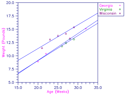
Figure 4, Plot of Turkey Weights and Fitted Lines by State
Example 2
A two-way analysis-of-variance model is fitted to balanced data discussed by Snedecor and Cochran (1967, Table 12.5.1, page 347). The responses are the weight gains (in grams) of rats fed diets varying in two components — level of protein and source of protein. The model is
yijk= μ + α i+ βj+ γij+ ɛ ijk i = 1, 2; j = 1, 2, 3; k = 1, 2, …, 10
where
Here, the IDUMMY = 0 option is used.
USE IMSL_LIBRARIES
IMPLICIT NONE
INTEGER IDEP, LDB, LDR, LDSCPE, LDX, LINDEF, MAXB, MAXCL, &
NCLVAR, NCOL, NEF, NROW
PARAMETER (IDEP=1, LINDEF=4, MAXB=12, MAXCL=5, NCLVAR=2, &
NCOL=3, NEF=3, NROW=60, LDB=MAXB, LDR=MAXB, &
LDSCPE=IDEP, LDX=NROW)
!
INTEGER I, IDUMMY, INDCL(NCLVAR), INDDEP(IDEP), &
INDEF(LINDEF), INTCEP, IRANK, IRBEF(NEF+1), J, &
NCLVAL(NCLVAR), NCOEF, NOUT, NRMISS, NVEF(NEF)
REAL B(LDB,IDEP), CLVAL(MAXCL), D(MAXB), DFE, &
R(LDR,MAXB), SCPE(LDSCPE,IDEP), X(LDX,NCOL), &
XMAX(MAXB), XMIN(MAXB)
CHARACTER CLABEL(MAXB+1)*7, RLABEL(1)*4
!
DATA X/73.0, 102.0, 118.0, 104.0, 81.0, 107.0, 100.0, 87.0, &
117.0, 111.0, 98.0, 74.0, 56.0, 111.0, 95.0, 88.0, 82.0, &
77.0, 86.0, 92.0, 94.0, 79.0, 96.0, 98.0, 102.0, 102.0, &
108.0, 91.0, 120.0, 105.0, 90.0, 76.0, 90.0, 64.0, 86.0, &
51.0, 72.0, 90.0, 95.0, 78.0, 107.0, 95.0, 97.0, 80.0, &
98.0, 74.0, 74.0, 67.0, 89.0, 58.0, 49.0, 82.0, 73.0, 86.0, &
81.0, 97.0, 106.0, 70.0, 61.0, 82.0, 30*1.0, 30*2.0, &
10*1.0, 10*2.0, 10*3.0, 10*1.0, 10*2.0, 10*3.0/
DATA INDCL/2, 3/, NVEF/1, 1, 2/, INDEF/2, 3, 2, 3/, INDDEP/1/
DATA CLABEL/' ', 'MU', 'ALPHA1', 'ALPHA2', 'BETA1', 'BETA2', &
'BETA3', 'GAMMA11', 'GAMMA12', 'GAMMA13', 'GAMMA21', &
'GAMMA22', 'GAMMA23'/
DATA RLABEL/'NONE'/
!
IDUMMY = 0
CALL RGLM (X, INDCL, NVEF, INDEF, IDEP, INDDEP, MAXCL, B, &
idummy=idummy, nclvar=nclvar, nclval=nclval, &
clval=clval, irbef=irbef, r=r, d=d, irank=irank, &
dfe=dfe, scpe=scpe, nrmiss=nrmiss, xmin=xmin, &
xmax=xmax)
!
CALL UMACH (2, NOUT)
WRITE (NOUT,*) 'NRMISS = ', NRMISS
WRITE (NOUT,*) 'IRANK = ', IRANK, ' DFE = ', DFE, ' '// &
'SCPE(1,1) = ', SCPE(1,1)
J = 0
DO 10 I=1, NCLVAR
CALL WRRRN ('Class Values', CLVAL((J+1):), 1, NCLVAL(I), 1)
J = J + NCLVAL(I)
10 CONTINUE
NCOEF = IRBEF(NEF+1) - 1
CALL WRRRN ('XMIN', XMIN, 1, NCOEF, 1)
CALL WRRRN ('XMAX', XMAX, 1, NCOEF, 1)
CALL WRIRN ('IRBEF', IRBEF, 1, NEF+1, 1)
CALL WRRRN ('R-MATRIX', R, NRA=NCOEF, NCA=NCOEF, ITRING=1)
CALL WRRRL ('B', B, RLABEL, CLABEL, 1, NCOEF, 1, FMT='(2W10.4)')
!
END
Output
NRMISS = 0
IRANK = 12 DFE = 54.0000 SCPE(1,1) = 11586.0
Class Values
1 2
1.000 2.000
Class Values
1 2 3
1.000 2.000 3.000
XMIN
1 2 3 4 5 6 7 8 9 10
1.000 0.000 0.000 0.000 0.000 0.000 0.000 0.000 0.000 0.000
11 12
0.000 0.000
XMAX
1 2 3 4 5 6 7 8 9 10
1.000 1.000 1.000 1.000 1.000 1.000 1.000 1.000 1.000 1.000
11 12
1.000 1.000
IRBEF
1 2 3 4
2 4 7 13
R-MATRIX
1 2 3 4 5 6 7 8 9
1 7.746 0.000 0.000 0.000 0.000 0.000 0.000 0.000 0.000
2 -1.000 -1.000 0.000 0.000 0.000 0.000 0.000 0.000
3 7.746 0.000 0.000 0.000 0.000 0.000 0.000
4 -1.000 -1.000 -1.000 0.000 0.000 0.000
5 6.325 3.162 0.000 0.000 0.000
6 5.477 0.000 0.000 0.000
7 -1.000 0.000 0.000
8 -1.000 0.000
9 -1.000
10 11 12
1 0.000 0.000 0.000
2 0.000 0.000 0.000
3 0.000 0.000 0.000
4 0.000 0.000 0.000
5 0.000 0.000 0.000
6 0.000 0.000 0.000
7 -1.000 0.000 0.000
8 0.000 -1.000 0.000
9 0.000 0.000 -1.000
10 -1.000 -1.000 -1.000
11 6.325 3.162
12 5.477
B
MU ALPHA1 ALPHA2 BETA1 BETA2 BETA3
87.87 7.267 -7.267 1.733 -2.967 1.233
GAMMA11 GAMMA12 GAMMA13 GAMMA21 GAMMA22 GAMMA23
3.133 -6.267 3.133 -3.133 6.267 -3.133


