RCASE
Computes case statistics and diagnostics given data points, coefficient estimates
and the R matrix for a fitted general linear model.
Required Arguments
X — NRX by NCOL matrix containing the data. (Input)
IRSP — Column number IRSP of X contains the data for the response (dependent) variable. (Input)
B — Vector of length NCOEF containing a least-squares solution
for the regression coefficients. (Input)
R — NCOEF by NCOEF upper triangular matrix containing the R matrix. (Input)
The R matrix can come from a regression fit based on a QR decomposition of the matrix of regressors or based on a Cholesky factorization RTR of the matrix of sums of squares and crossproducts of the regressors. Elements to the right of a diagonal element of R that is zero must also be zero. A zero row indicates a nonfull rank model. For an R matrix that comes from a regression fit with linear equality restrictions on the parameters, each row of R corresponding to a restriction must have a corresponding diagonal element that is negative. The remaining rows of R must have positive diagonal elements. Only the upper triangle of R is referenced.
The R matrix can come from a regression fit based on a QR decomposition of the matrix of regressors or based on a Cholesky factorization RTR of the matrix of sums of squares and crossproducts of the regressors. Elements to the right of a diagonal element of R that is zero must also be zero. A zero row indicates a nonfull rank model. For an R matrix that comes from a regression fit with linear equality restrictions on the parameters, each row of R corresponding to a restriction must have a corresponding diagonal element that is negative. The remaining rows of R must have positive diagonal elements. Only the upper triangle of R is referenced.
DFE — Degrees of freedom for error. (Input)
SSE — Sum of squares for error. (Input)
CASE — NRX by 12 matrix containing the case statistics. (Output)
Columns 1 through 12 contain the following:
Columns 1 through 12 contain the following:
Col. | Description |
1 | Observed response |
2 | Predicted response |
3 | Residual |
4 | Leverage |
5 | Standardized residual |
6 | Jackknife residual |
7 | Cook’s distance |
8 | DFFITS |
9, 10 | Confidence interval on the mean |
11, 12 | Prediction interval |
Optional Arguments
IDO — Processing option. (Input)
Default: IDO = 0.
Default: IDO = 0.
IDO | Action |
0 | This is the only invocation of RCASE for this data set, and all the data are input at once. |
1 | This is the first invocation, and additional calls to RCASE will be made. Case statistics are computed for the data in X. |
2 | This is an intermediate or final invocation of RCASE. Case statistics are computed for the data in X. |
NRX — Number of rows in X. (Input)
Default: NRX = size (X,1).
Default: NRX = size (X,1).
NCOL — Number of columns in X. (Input)
Default: NCOL = size (X,2).
Default: NCOL = size (X,2).
LDX — Leading dimension of X exactly as specified in the dimension statement in the calling program. (Input)
Default: LDX = size (X,1).
Default: LDX = size (X,1).
INTCEP — Intercept option. (Input)
Default: INTCEP = 1.
Default: INTCEP = 1.
INTCEP | Action |
|---|---|
0 | An intercept is not in the model. |
1 | An intercept is in the model. |
IEF — Effect option. (Input)
Default: IEF = ‑1.
The absolute value of IEF is the number of effects (sources of variation) due to the model. The sign of IEF specifies the following options.
Default: IEF = ‑1.
The absolute value of IEF is the number of effects (sources of variation) due to the model. The sign of IEF specifies the following options.
IEF | Meaning |
|---|---|
< 0 | Each effect corresponds to a single regressor (coefficient) in the model. In this case, arguments NCLVAR, INDCL, NCLVAL, CLVAL, NVEF, INDEF, and IDUMMY are not referenced. |
> 0 | Each effect corresponds to one or more regressors. A general linear model is specified through the arguments NCLVAR, INDCL, NCLVAL, CLVAL, NVEF, INDEF, and IDUMMY. |
0 | There are no effects in the model. INTCEP must equal 1. |
NCLVAR — Number of classification variables. (Input, if IEF is positive)
INDCL — Index vector of length NCLVAR containing the column numbers of X that are the classification variables. (Input, if IEF is positive)
NCLVAL — Vector of length NCLVAR containing the number of values taken on by each classification variable. (Input, if IEF is positive)
NCLVAL(I) is the number of distinct values for the I-th classification variable.
NCLVAL(I) is the number of distinct values for the I-th classification variable.
CLVAL — Vector of length NCLVAL(1) + NCLVAL(2) + … + NCLVAL(NCLVAR) containing the values of the classification variables. (Input, if IEF is positive)
The first NCLVAL(1) variables contain the values of the first classification variable; the next NCLVAL(2) variables contain the values of the second classification variable; and so on. The last NCLVAL(NCLVAR) variables contain the values of the last classification variable.
The first NCLVAL(1) variables contain the values of the first classification variable; the next NCLVAL(2) variables contain the values of the second classification variable; and so on. The last NCLVAL(NCLVAR) variables contain the values of the last classification variable.
NVEF — Vector of length IEF containing the number of variables associated with each effect in the model. (Input, if IEF is positive)
INDEF — Index vector of length NVEF(1) + NVEF(2) + … + NVEF(IEF). (Input, if IEF is positive)
The first NVEF(1) elements give the column numbers of X for each variable in the first effect; the next NVEF(2) elements give the column numbers for each variable in the second effect; and so on. The last NVEF(NEF) elements give the column numbers for each variable in the last effect.
The first NVEF(1) elements give the column numbers of X for each variable in the first effect; the next NVEF(2) elements give the column numbers for each variable in the second effect; and so on. The last NVEF(NEF) elements give the column numbers for each variable in the last effect.
IDUMMY — Dummy variable option. (Input, if IEF is positive)
Some indicator variables are defined for the I-th class variable as follows: Let J = NCLVAL(1) + NCLVAL(2) + … + NCLVAL(I ‑ 1). NCLVAL(I) indicator variables are defined such that for K = 1, 2, …, NCLVAL(I) the K-th indicator variable for row M of X takes the value 1.0 if X(M, INDCL(I)) = CLVAL(J + K) and equals 0.0 otherwise. Dummy variables are generated from these indicator variables in one of the three following ways:
Some indicator variables are defined for the I-th class variable as follows: Let J = NCLVAL(1) + NCLVAL(2) + … + NCLVAL(I ‑ 1). NCLVAL(I) indicator variables are defined such that for K = 1, 2, …, NCLVAL(I) the K-th indicator variable for row M of X takes the value 1.0 if X(M, INDCL(I)) = CLVAL(J + K) and equals 0.0 otherwise. Dummy variables are generated from these indicator variables in one of the three following ways:
IDUMMY | Method |
|---|---|
0, 1 | The NCLVAL(I) indicator variables are the dummy variables (In RCASE, the computations for IDUMMY = 0 and IDUMMY = 1 are the same. The two values 0 and 1 are provided so that RCASE can be called after routine RGLM with no change in IDUMMY.) |
2 | The first NCLVAL(I) ‑ 1 indicator variables are the dummy variables. The last indicator variable is omitted. |
3 | The K-th indicator variable minus the NCLVAL (I)-th indicator variable is the K-th dummy variable (K = 1, 2, …, NCLVAL(I) ‑ 1). |
IWT — Weighting option. (Input)
IWT = 0 means that all weights are 1.0. For positive IWT, column number IWT of X contains the weights, and the computed prediction interval uses SSE/(DFE * X(I, IWT)) for the estimated variance of a future response.
Default: IWT = 0.
IWT = 0 means that all weights are 1.0. For positive IWT, column number IWT of X contains the weights, and the computed prediction interval uses SSE/(DFE * X(I, IWT)) for the estimated variance of a future response.
Default: IWT = 0.
IPRED — Prediction interval option. (Input)
IPRED = 0 means that prediction intervals are desired for a single future response. For positive IPRED, column number IPRED of X contains the number of future responses for which a prediction interval is desired on the average of the future responses.
Default: IPRED = 0.
IPRED = 0 means that prediction intervals are desired for a single future response. For positive IPRED, column number IPRED of X contains the number of future responses for which a prediction interval is desired on the average of the future responses.
Default: IPRED = 0.
CONPCM — Confidence level for two-sided interval estimates on the mean, in percent. (Input)
CONPCM percent confidence intervals are computed, hence, CONPCM must be greater than or equal to 0.0 and less than 100.0. CONPCM often will be 90.0, 95.0, or 99.0. For one-sided intervals with confidence level ONECL, where ONECL is greater than or equal to 50.0 and less than 100.0, set CONPCM = 100.0 ‑ 2.0 * (100.0 ‑ ONECL).
Default: CONPCM = 95.0.
CONPCP — Confidence level for two-sided prediction intervals, in percent. (Input)
CONPCP percent prediction intervals are computed, hence, CONPCP must be greater than or equal to 0.0 and less than 100.0. CONPCP often will be 90.0, 95.0, or 99.0. For one-sided intervals with confidence level ONECL, where ONECL is greater than or equal to 50.0 and less than 100.0, set CONPCP = 100.0 ‑ 2.0 * (100.0 ‑ ONECL).
Default: CONPCP = 95.0.
PRINT — Printing option. (Input)
Default: PRINT = ‘N’.
PRINT is a character string indicating what is to be printed. The PRINT string is composed of one-character print codes to control printing. These print codes are given as follows:
Default: PRINT = ‘N’.
PRINT is a character string indicating what is to be printed. The PRINT string is composed of one-character print codes to control printing. These print codes are given as follows:
PRINT(I:I) | Printing that Occurs |
|---|---|
‘A’ | All |
‘N’ | None |
‘1’ | Observed response |
‘2’ | Predicted response |
‘3’ | Residual |
‘4’ | Leverage |
‘5’ | Standardized residual |
‘6’ | Jackknife residual |
‘7’ | Cook’s distance |
‘8’ | DFFITS |
‘M’ | Confidence interval on the mean |
‘P’ | Prediction interval |
‘X’ | Influential cases (unusual “x‑value”) |
‘Y’ | Outlier cases (unusual “y‑value”) |
The concatenated print codes ‘A’, ‘N’, ‘1’, …, ‘P’ that comprise the PRINT string give the combination of statistics to be printed. Concatenation of these codes with print codes ‘X’ or ‘Y’ restricts printing to cases determined to be influential or outliers. Here are a few examples.
PRINT | Printing Action |
‘A’ | All. |
‘N’ | None. |
‘46’ | Leverage and jackknife residual for all cases. |
‘AXY’ | All statistics are printed for cases that are highly influential or are outliers. |
‘46XY’ | Leverage and jackknife residual are printed for cases that are highly influential or are outliers. |
IOBS — Number of the observation corresponding to the first row of X. (Input)
This observation number is used only for printing the row labels for the individual case statistics.
Default: IOBS = size (X,1).
This observation number is used only for printing the row labels for the individual case statistics.
Default: IOBS = size (X,1).
NCOEF — Number of regression coefficients in the model. (Input)
Default: NCOEF = size (B,1).
Default: NCOEF = size (B,1).
LDR — Leading dimension of R exactly as specified in the dimension statement in the calling program. (Input)
Default: LDR = size (R,1).
Default: LDR = size (R,1).
LDCASE — Leading dimension of CASE exactly as specified in the dimension statement in the calling program. (Input)
Default: LDCASE = size (CASE,1).
Default: LDCASE = size (CASE,1).
NRMISS — Number of rows of CASE containing NaN (not a number). (Output)
If any row of data contains NaN as a value of a variable other than the response variable, columns 3 through 12 of the corresponding row in CASE are set to NaN. If the response is missing, columns 1, 3, and 5 through 8 are set to NaN.
If any row of data contains NaN as a value of a variable other than the response variable, columns 3 through 12 of the corresponding row in CASE are set to NaN. If the response is missing, columns 1, 3, and 5 through 8 are set to NaN.
FORTRAN 90 Interface
Generic: CALL RCASE (X, IRSP, B, R, DFE, SSE, CASE [, …])
Specific: The specific interface names are S_RCASE and D_RCASE.
FORTRAN 77 Interface
Single: CALL RCASE (IDO, NRX, NCOL, X, LDX, INTCEP, IEF, NCLVAR, INDCL, NCLVAL, CLVAL, NVEF, INDEF, IDUMMY, IRSP, IWT, IPRED, CONPCM, CONPCP, PRINT, IOBS, NCOEF, B, R, LDR, DFE, SSE, CASE, LDCASE, NRMISS)
Double: The double precision name is DRCASE.
Description
The general linear model used by routine RCASE is
y = X β + ɛ
where y is the n × 1 vector of responses, X is the n × p matrix of regressors, β is the p × 1 vector of regression coefficients, and ɛ is the n × 1 vector of errors whose elements are independently normally distributed with mean 0 and variance σ2/wi. The model used by RCASE also permits linear equality restrictions on β. From a general linear model fitted using the wi’s as the weights, routine RCASE computes confidence intervals and statistics for the individual cases that constitute the data set. Let xi be a column vector containing elements of the i-th row of X. Let W = diag(w1, w2, …, wn). The leverage is defined as
(In the case of linear equality restrictions on β, the leverage is defined in terms of the reduced model.) Put D = diag(d1, d2, …, dp) with dj = 1 if the j-th diagonal element of R is positive and 0 otherwise. The leverage is computed as hi = (aTDa)wi where a is a solution to RTa = xi. The estimated variance of
is given by his2/wi, where s2 = SSE/DFE. The computation of the remainder of the case statistics follows easily from their definitions. See the Diagnostics for Individual Cases section in the chapter introduction for definitions of the case diagnostics.
Often predicted values and confidence intervals are desired for combinations of settings of the effect variables not used in computing the regression fit. This can be accomplished using a single data matrix by including these settings of the variables as part of the data matrix and by setting the response equal to NaN (not a number). NaN can be retrieved by the invocation of the function AMACH(6). The regression routine performing the fit will omit the case, and RCASE will compute a predicted value and confidence interval for the missing response from the given settings of the effect variables.
The type 3 informational errors can occur if the input variables X, R, B and SSE are not consistent with each other or if excessive rounding has occurred in their computation. The type 3 error message with error code 2 arises when X contains a row not in the space spanned by the rows of R. An examination of the model that was fitted and the X for which diagnostics are to be computed is required in order to insure that only linear combinations of the regression coefficients that can be estimated from the fitted model are specified in X. For further details, see the discussion of estimable functions given by Maindonald (1984, pages 166‑168) and Searle (1971, pages 180‑188).
Comments
1. Workspace may be explicitly provided, if desired, by use of R2ASE/DR2ASE. The reference is:
CALL R2ASE (IDO, NRX, NCOL, X, LDX, INTCEP, IEF, NCLVAR, INDCL, NCLVAL, CLVAL, NVEF, INDEF, IDUMMY, IRSP, IWT, IPRED, CONPCM, CONPCP, PRINT, IOBS, NCOEF, B, R, LDR, DFE, SSE, CASE, LDCASE, NRMISS, WK)
The additional argument is:
WK — Work vector of length NCOEF + 1.
2. Informational errors
Type | Code | Description |
|---|---|---|
4 | 1 | A weight is negative. Weights must be nonnegative. |
3 | 2 | The linear combination of the regression coefficients specified is not estimable within the preset tolerance. |
3 | 3 | A leverage much greater than 1.0 was computed. It is set to 1.0. |
3 | 4 | A deleted residual mean square much less than 0.0 was computed. It is set to 0.0. |
4 | 5 | A number of future observations for the prediction interval is nonpositive. It must be positive. |
Examples
Example 1
A multiple linear regression model is fitted and case statistics computed for data discussed by Cook and Weisberg (1982, page 103). The fitted model is
Some of the statistics in row 6 of the output matrix CASE are undefined (0.0/0.0) and are set to NaN (not a number). Some statistics in row 4 of CASE are set to Inf (positive machine infinity). The values of NaN and positive machine infinity can be retrieved by routine AMACH (or DMACH when using double precision), which is documented in the section “Machine-Dependent Constants” in Reference Material.
USE RCASE_INT
USE RGIVN_INT
IMPLICIT NONE
INTEGER INTCEP, LDB, LDCASE, LDR, LDSCPE, LDX, NCOEF, NCOL, &
NDEP, NIND, NROW, J, NRMISS
PARAMETER (INTCEP=1, NCOL=3, NDEP=1, NIND=2, NROW=7, &
LDCASE=NROW, LDSCPE=NDEP, LDX=NROW, &
NCOEF=INTCEP+NIND, LDB=NCOEF, LDR=NCOEF)
!
INTEGER IDEP, IEF, IIND, INDDEP(1), INDIND(1), IOBS, IRSP
REAL B(LDB,NDEP), CASE(LDCASE,12), DFE, R(LDR,NCOEF), &
SCPE(LDSCPE,NDEP), SSE, X(LDX,NCOL)
CHARACTER PRINT*1
!
DATA (X(1,J),J=1,NIND+NDEP) /1.0, 1.0, 3.0/
DATA (X(2,J),J=1,NIND+NDEP) /1.0, 2.0, 4.0/
DATA (X(3,J),J=1,NIND+NDEP) /1.0, 3.0, 5.0/
DATA (X(4,J),J=1,NIND+NDEP) /1.0, 4.0, 7.0/
DATA (X(5,J),J=1,NIND+NDEP) /1.0, 5.0, 7.0/
DATA (X(6,J),J=1,NIND+NDEP) /0.0, 6.0, 8.0/
DATA (X(7,J),J=1,NIND+NDEP) /1.0, 7.0, 9.0/
!
IIND = -NIND
IDEP = -NDEP
CALL RGIVN (X, IIND, INDIND, IDEP, INDDEP, B, R=R, DFE=DFE, SCPE=SCPE)
IEF = -NIND
IRSP = NCOL
PRINT = 'A'
IOBS = 1
SSE = SCPE(1,1)
CALL RCASE (X, IRSP, B(1:,1), R, DFE, SSE, CASE, ief=ief, &
PRINT=PRINT, iobs=iobs, ncoef=ncoef, nrmiss=nrmiss)
!
END
Output
* * * Case Analysis * * *
Obs. Observed Predicted Residual Leverage Std. Res. Jack Res.
Cook’s D DFFITS 95.0% CI 95.0% CI 95.0% PI 95.0% PI
1 3.0000 3.1286 -0.1286 0.4714 -0.3886 -0.3430
0.0449 -0.3240 2.2609 3.9962 1.5957 4.6614
2 4.0000 4.1429 -0.1429 0.2857 -0.3714 -0.3273
0.0184 -0.2070 3.4674 4.8183 2.7100 5.5757
3 5.0000 5.1571 -0.1571 0.1857 -0.3826 -0.3376
0.0111 -0.1612 4.6126 5.7017 3.7812 6.5331
Y 4 7.0000 6.1714 0.8286 0.1714 2.0000 Inf
0.2759 Inf 5.6482 6.6946 4.8038 7.5391
5 7.0000 7.1857 -0.1857 0.2429 -0.4689 -0.4178
0.0235 -0.2366 6.5630 7.8084 5.7770 8.5945
X 6 8.0000 8.0000 0.0000 1.0000 NaN NaN
NaN NaN 6.7364 9.2636 6.2129 9.7871
7 9.0000 9.2143 -0.2143 0.6429 -0.7878 -0.7423
0.3724 -0.9959 8.2011 10.2275 7.5946 10.8339
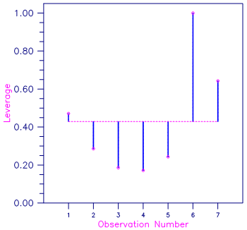
Figure 6, Plot of Leverages hi and the Average (p/n = 3/7)
Example 2
A one-way analysis of covariance model is fitted to the turkey data discussed by Draper and Smith (1981, pages 243‑249). The response variable is turkey weight y (in pounds). There are three groups of turkeys corresponding to the three states where they were reared. The age of a turkey (in weeks) is the covariate. The explanatory variables are group, age, and interaction. The model is
where α3 = 0 and β3 = 0. Routine RGLM is used to fit the model. The option IDUMMY = 2 is used. The fitted model gives three separate lines, one for each state where the turkeys were reared. Then, RCASE is used to compute case statistics from the fitted model.
USE RCASE_INT
USE RGLM_INT
USE AMACH_INT
INTEGER IDEP, IEF, INTCEP, LDB, LDCASE, LDR, LDSCPE, LDX, &
MAXB, MAXCL, NCLVAR, NCOL, NROW
PARAMETER (IDEP=1, IEF=3, INTCEP=1, MAXB=6, MAXCL=3, NCLVAR=1, &
NCOL=3, NROW=13, LDB=MAXB, LDCASE=NROW, LDR=MAXB, &
LDSCPE=IDEP, LDX=NROW)
!
INTEGER IDUMMY, INDCL(NCLVAR), INDDEP(IDEP), &
INDEF(4), IOBS, IRANK, IRBEF(IEF+1), IRSP, &
NCLVAL(NCLVAR), NCOEF, NRMISS, NVEF(IEF)
REAL B(LDB,IDEP), CASE(LDCASE,12), CLVAL(MAXCL), &
DFE, R(LDR,MAXB),SCPE(LDSCPE,IDEP), SSE, X(LDX,NCOL)
CHARACTER PRINT
!
DATA (X(1,J),J=1,3) /25.0, 13.8, 3.0/
DATA (X(2,J),J=1,3) /28.0, 13.3, 1.0/
DATA (X(3,J),J=1,3) /20.0, 8.9, 1.0/
DATA (X(4,J),J=1,3) /32.0, 15.1, 1.0/
DATA (X(5,J),J=1,3) /22.0, 10.4, 1.0/
DATA (X(6,J),J=1,3) /29.0, 13.1, 2.0/
DATA (X(7,J),J=1,3) /27.0, 12.4, 2.0/
DATA (X(8,J),J=1,3) /28.0, 13.2, 2.0/
DATA (X(9,J),J=1,3) /26.0, 11.8, 2.0/
DATA (X(10,J),J=1,3) /21.0, 11.5, 3.0/
DATA (X(11,J),J=1,3) /27.0, 14.2, 3.0/
DATA (X(12,J),J=1,3) /29.0, 15.4, 3.0/
DATA (X(13,J),J=1,3) /23.0, 13.1, 3.0/
DATA INDCL/3/, NVEF/1, 1, 2/, INDEF/3, 1, 1, 3/, INDDEP/2/
!
IDUMMY = 2
CALL RGLM (X, INDCL, NVEF, INDEF, IDEP, INDDEP, MAXCL, B, &
IDUMMY=IDUMMY, NCLVAL=NCLVAL, CLVAL=CLVAL, IRBEF=IRBEF, &
R=R, DFE=DFE, SCPE=SCPE)
!
PRINT = 'A'
IRSP = INDDEP(1)
IPRED = 0
PRINT = 'A'
IOBS = 1
NCOEF = IRBEF(IEF+1) - 1
SSE = SCPE(1,1)
CALL RCASE (X, IRSP, B(1:, 1), R, DFE, SSE, CASE, IEF=IEF, &
NCLVAR=NCLVAR, INDCL=INDCL, NCLVAL=NCLVAL, CLVAL=CLVAL, &
NVEF=NVEF, INDEF=INDEF, IDUMMY=IDUMMY, IOBS=IOBS, &
PRINT=PRINT, NCOEF=NCOEF)
!
END
Output
* * * Case Analysis * * *
Obs. Observed Predicted Residual Leverage Std. Res. Jack Res.
Cook’s D DFFITS 95.0% CI 95.0% CI 95.0% PI 95.0% PI
1 13.8000 13.6000 0.2000 0.2000 0.7040 0.6762
0.0207 0.3381 13.2641 13.9359 12.7773 14.4227
2 13.3000 13.1901 0.1099 0.3187 0.4192 0.3930
0.0137 0.2688 12.7661 13.6141 12.3276 14.0526
3 8.9000 9.1418 -0.2418 0.5824 -1.1779 -1.2178
0.3225 -1.4383 8.5686 9.7149 8.1970 10.0865
4 15.1000 15.2143 -0.1143 0.7143 -0.6732 -0.6444
0.1888 -1.0189 14.5795 15.8490 14.2309 16.1976
5 10.4000 10.1538 0.2462 0.3846 0.9879 0.9860
0.1017 0.7795 9.6881 10.6196 9.2701 11.0376
6 13.1000 13.3300 -0.2300 0.7000 -1.3221 -1.4131
0.6797 -2.1585 12.7016 13.9584 12.3507 14.3093
7 12.4000 12.3900 0.0100 0.3000 0.0376 0.0348
0.0001 0.0228 11.9786 12.8014 11.5337 13.2463
8 13.2000 12.8600 0.3400 0.3000 1.2795 1.3533
0.1169 0.8859 12.4486 13.2714 12.0037 13.7163
9 11.8000 11.9200 -0.1200 0.7000 -0.6898 -0.6615
0.1850 -1.0104 11.2916 12.5484 10.9407 12.8993
10 11.5000 11.8200 -0.3200 0.6000 -1.5930 -1.8472
0.6344 -2.2623 11.2382 12.4018 10.8700 12.7700
11 14.2000 14.4900 -0.2900 0.3000 -1.0913 -1.1091
0.0851 -0.7261 14.0786 14.9014 13.6337 15.3463
12 15.4000 15.3800 0.0200 0.6000 0.0996 0.0922
0.0025 0.1130 14.7982 15.9618 14.4300 16.3300
13 13.1000 12.7100 0.3900 0.3000 1.4676 1.6330
0.1538 1.0691 12.2986 13.1214 11.8537 13.5663


