-
Interface Summary Interface Description Activation Interface implemented by perceptron activation functions.QuasiNewtonTrainer.Error Error function to be minimized by trainer.Trainer Interface implemented by classes used to train a network. -
Class Summary Class Description BinaryClassification Classifies patterns into two classes.EpochTrainer Performs two-stage training using randomly selected training patterns in stage I.FeedForwardNetwork A representation of a feed forward neural network.HiddenLayer Hidden layer in a neural network.InputLayer Input layer in a neural network.InputNode ANodein theInputLayer.Layer The base class forLayers in a neural network.LeastSquaresTrainer Trains aFeedForwardNetworkusing a Levenberg-Marquardt algorithm for minimizing a sum of squares error.Link A link in a neural network.MultiClassification Classifies patterns into three or more classes.Network Neural network base class.Node ANodein a neural network.OutputLayer Output layer in a neural network.OutputPerceptron APerceptronin theOutputLayer.Perceptron APerceptronnode in a neural network.QuasiNewtonTrainer Trains a network using the quasi-Newton method,MinUnconMultiVar.ScaleFilter Scales or unscales continuous data prior to its use in neural network training, testing, or forecasting.TimeSeriesClassFilter Converts time series data contained within nominal categories to a lagged format for processing by a neural network.TimeSeriesFilter Converts time series data to a lagged format used as input to a neural network.Trace Standardizes the output format for the neural network log files.UnsupervisedNominalFilter Converts nominal data into a series of binary encoded columns for input to a neural network.UnsupervisedOrdinalFilter Encodes ordinal data into percentages for input to a neural network.
Package com.imsl.datamining.neural Description
Overview of Neural Networks
Today, neural networks are used to solve a wide variety of problems, some of which have been solved by existing statistical methods, and some of which have not. These applications fall into one of the following three categories:
- Forecasting: predicting one or more quantitative outcomes from both quantitative and categorical input data,
- Classification: classifying input data into one of two or more categories, or
- Statistical pattern recognition: uncovering patterns, typically spatial or temporal, among a set of variables.
Forecasting, pattern recognition and classification problems are not new. They existed years before the discovery of neural network solutions in the 1980's. What is new is that neural networks provide a single framework for solving so many traditional problems and, in some cases, extend the range of problems that can be solved.
Traditionally, these problems have been solved using a variety of well known statistical methods:
- linear regression and general least squares,
- logistic regression and discrimination,
- principal component analysis,
- discriminant analysis,
- k-nearest neighbor classification, and
- ARMA and non-linear ARMA time series forecasts.
In many cases, simple neural network configurations yield the same solution as many traditional statistical applications.For example, a single-layer, feed-forward neural network with linear activation for its output perceptron is equivalent to a general linear regression fit. Neural networks can provide more accurate and robust solutions for problems where traditional methods do not completely apply.
Mandic and Chambers (2001) point out that traditional methods for time series forecasting are unsuitable when a time series:
- is non-stationary,
- has large amounts of noise, such as a biomedical series, or
- is too short.
ARIMA and other traditional time series approaches can produce poor forecasts when one or more of the above problems exist. The forecasts of ARMA and non-linear ARMA (NARMA) depend heavily upon key assumptions about the model or underlying relationship between the output of the series and its patterns.
Neural networks, on the other hand, adapt to changes in a non-stationary series and can produce reliable forecasts even when the series contains a good deal of noise or when only a short series is available for training. Neural networks provide a single tool for solving many problems traditionally solved using a wide variety of statistical tools and for solving problems when traditional methods fail to provide an acceptable solution.
Although neural network solutions to forecasting, pattern recognition, and classification problems can be very different, they are always the result of computations that proceed from the network inputs to the network outputs. The network inputs are referred to as patterns, and outputs are referred to as classes. Frequently the flow of these computations is in one direction, from the network input patterns to its outputs. Networks with forward-only flow are referred to as feed-forward networks.
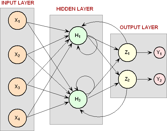
Other networks, such as recurrent neural networks, allow data and information to flow in both directions, see Mandic and Chambers (2001).
A neural network is defined not only by its architecture and flow, or interconnections, but also by computations used to transmit information from one node or input to another node. These computations are determined by network weights. The process of fitting a network to existing data to determine these weights is referred to as training the network, and the data used in this process are referred to as patterns. Individual network inputs are referred to as attributes and outputs are referred to as classes. Many terms used to describe neural networks are synonymous to common statistical terminology.
| Neural Network Terminology | Traditional Statistical Terminology | Description |
| Training | Model Fitting | Estimating unknown parameters or coefficients in the analysis. |
| Patterns | Cases or Observations | A single observation of all input and output variables. |
| Attributes | Independent variables | Inputs to the network or model. |
| Classes | Dependent variables | Outputs from the network or model calculations. |
Neural Networks -- History and Terminology
The Threshold Neuron
McCulloch and Pitts (1943) wrote one of the first published works on neural networks. In their paper, they describe the threshold neuron as a model for how the human brain stores and processes information.
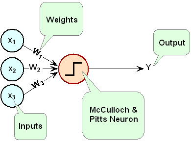
All inputs to a threshold neuron are combined into a single number, Z, using the following weighted sum: \(Z = \sum\limits_{i = 1}^m {w_i x_i } - \mu\) where \(w_i\) is the weight associated with the i-th input (attribute) \(x_i\). The term \(\mu\) in this calculation is referred to as the bias term. In traditional statistical terminology, it might be referred to as the intercept. The weights and bias terms in this calculation are estimated during network training.
In McCulloch and Pitt's description of the threshold neuron, the neuron does not respond to its inputs unless Z is greater than zero. If Z is greater than zero then the output from this neuron is set equal to 1. If Z is less than zero the output is zero: $$ Y=\left\{{\begin{array}{*{20}c}1&{{\text{if }} Z>0}\\0&{{\text{if }} Z\le0}\\\end{array}}\right.$$ where Y is the neuron's output.
For years following their 1943 paper, interest in the McCulloch and Pitts neural network was limited to theoretical discussions, such as those of Hebb (1949), about learning, memory, and the brain's structure.
The Perceptron
The McCulloch and Pitts neuron is also referred to as a threshold neuron since it abruptly changes its output from 0 to 1 when its potential, Z, crosses a threshold. Mathematically, this behavior can be viewed as a step function that maps the neuron's potential, Z, to the neuron's output, Y.
Rosenblatt (1958) extended the McCulloch and Pitts threshold neuron by replacing this step function with a continuous function that maps Z to Y. The Rosenblatt neuron is referred to as the perceptron, and the continuous function mapping Z to Y makes it easier to train a network of perceptrons than a network of threshold neurons.
Unlike the threshold neuron, the perceptron produces analog output rather than the threshold neuron's purely binary output. Carefully selecting the analog function makes Rosenblatt's perceptron differentiable, whereas the threshold neuron is not. This simplifies the training algorithm.
Like the threshold neuron, Rosenblatt's perceptron starts by calculating a weighted sum of its inputs, \(Z=\sum\limits_{i=1}^m{w_i x_i}-\mu\). This is referred to as the perceptron's potential.
Rosenblatt's perceptron calculates its analog output from its potential. There are many choices for this calculation. The function used for this calculation is referred to as the activation function in Figure 4 below.
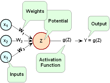
As shown in Figure 4, perceptrons consist of the following five components:
| Component | Example |
| Inputs | \(X_1, X_2, X_3\), |
| Input Weights | \(W_1,W_2,W_3\), |
| Potential | \(Z =\sum\limits_{i=1}^3{W_i}X_i-\mu\), where \(\mu\) is a bias correction. |
| Activation Function | \(g()\) |
| Output | \(g(Z)\) |
Like threshold neurons, perceptron inputs can be either the initial raw data inputs or the output from another perceptron. The primary purpose of the network training is to estimate the weights associated with each perceptron's potential. The activation function maps this potential to the perceptron's output.
The Activation Function
Although theoretically any differential function can be used as an activation function, the identity and sigmoid functions are the two most commonly used.
The identity activation function, also referred to as a linear activation function, is a flow-through mapping of the perceptron's potential to its output: \(g\left( Z \right) = Z\)
Output perceptrons in a forecasting network often use the identity activation function.
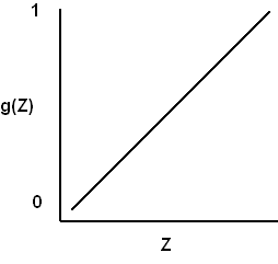
If the identity activation function is used throughout the network, then it is easily shown that the network is equivalent to fitting a linear regression model of the form \(Y_i=\beta_0+\beta_1x_1+\cdots+\beta_kx_k\), where \(x_1,x_2,\cdots,x_k\) are the \(k\) network inputs, \(Y_i\) is the i-th network output and \(\beta_0,\beta_1,\cdots,\beta_k\) are the coefficients in the regression equation. As a result, it is uncommon to find a neural network with identity activation used in all its perceptrons.
Sigmoid activation functions are differentiable functions that map the perceptron's potential to a range of values, such as 0 to 1, i.e., \(\mathbb{R}^K\to\mathbb{R}\) where K is the number of perceptron inputs.
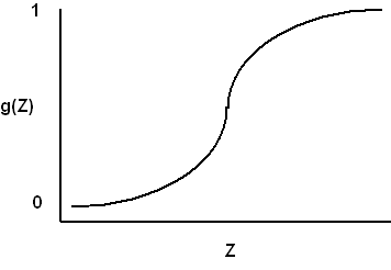
In practice, the most common sigmoid activation function is the logistic function that maps the potential into the range 0 to 1:
$$g(Z) = \frac{1}{{1+e^{-Z}}}$$Since \(0 \lt g(Z) \lt 1\), the logistic function is very popular for use in networks that output probabilities.
Other popular sigmoid activation functions include:
- the hyperbolic-tangent $$ g(Z)=\tanh (Z)=\frac{{e^{\alpha Z}- e^{-\alpha Z} }}{{e^{\alpha Z}+e^{-\alpha Z} }}$$
- the arc-tangent $$ g(Z)={\textstyle{2\over\pi }}\arctan\left({\frac{{\pi Z}}{2}}\right)$$
- the squash activation function (Elliott (1993)) $$ g(Z)=\frac{Z}{{1+\left|Z\right|}}$$
It is easy to show that the hyperbolic-tangent and logistic activation functions are linearly related. Consequently, forecasts produced using logistic activation should be close to those produced using hyperbolic-tangent activation. However, one function may be preferred over the other when training performance is a concern. Researchers report that the training time using the hyperbolic-tangent activation function is shorter than using the logistic activation function.
Network Applications
Forecasting using Neural Networks
There are many good statistical forecasting tools. Most require assumptions about the relationship between the variables being forecasted and the variables used to produce the forecast, as well as the distribution of forecast errors. Such statistical tools are referred to as parametric methods. ARIMA time series models, for example, assume that the time series is stationary, that the errors in the forecasts follow a particular ARIMA model, and that the probability distribution for the residual errors is Gaussian, see Box and Jenkins (1970). If these assumptions are invalid, then ARIMA time series forecasts can be very poor.
Neural networks, on the other hand, require few assumptions. Since neural networks can approximate highly non-linear functions, they can be applied without an extensive analysis of underlying assumptions.
Another advantage of neural networks over ARIMA modeling is the number of observations needed to produce a reliable forecast. ARIMA models generally require 50 or more equally spaced, sequential observations in time. In many cases, neural networks can also provide adequate forecasts with fewer observations by incorporating exogenous, or external, variables in the network's input.
For example, a company applying ARIMA time series analysis to forecast business expenses would normally require each of its departments, and each sub-group within each department to prepare its own forecast. For large corporations this can require fitting hundreds or even thousands of ARIMA models. With a neural network approach, the department and sub-group information could be incorporated into the network as exogenous variables. Although this can significantly increase the network's training time, the result would be a single model for predicting expenses within all departments and sub-departments.
Linear least squares models are also popular statistical forecasting tools. These methods range from simple linear regression for predicting a single quantitative outcome to logistic regression for estimating probabilities associated with categorical outcomes. It is easy to show that simple linear least squares forecasts and logistic regression forecasts are equivalent to a feed-forward network with a single layer. For this reason, single-layer feed-forward networks are rarely used for forecasting. Instead multilayer networks are used.
Hutchinson (1994) and Masters (1995) describe using multilayer feed-forward neural networks for forecasting. Multilayer feed-forward networks are characterized by the forward-only flow of information in the network. The flow of information and computations in a feed-forward network is always in one direction, mapping an \(M\)-dimensional vector of inputs to a \(C\)-dimensional vector of outputs, i.e., $$\mathbb{R}^M\to\mathbb{R}^C$$
There are many other types of networks without this feed-forward requirement. Information and computations in a recurrent neural network, for example, flow in both directions. Output from one level of a recurrent neural network can be fed back, with some delay, as input into the same network, see Figure 2. Recurrent networks are very useful for time series prediction, see Mandic and Chambers (2001).
Pattern Recognition using Neural Networks
Neural networks are also extensively used in statistical pattern recognition. Pattern recognition applications that make wide use of neural networks include:
- natural language processing: Manning and Schütze (1999)
- speech and text recognition: Lippmann (1989)
- face recognition: Lawrence, et al. (1997)
- playing backgammon, Tesauro (1990)
- classifying financial news, Calvo (2001).
The interest in pattern recognition using neural networks has stimulated the development of important variations of feed-forward networks. Two of the most popular are:
- Self-Organizing Maps, also called Kohonen Networks, Kohonen (1995),
- and Radial Basis Function Networks, Bishop (1995).
Good mathematical descriptions of the neural network methods underlying these applications are given by Bishop (1995), Ripley (1996), Mandic and Chambers (2001), and Abe (2001). An excellent overview of neural networks, from a statistical viewpoint, is also found in Warner and Misra (1996).
Neural Networks for Classification
Classifying observations using prior concomitant information is a popular application of neural networks. Data classification problems abound in business and research. When decisions based upon data are needed, they can often be treated as a neural network data classification problem. Decisions to buy, sell, hold or do nothing with a stock, are decisions involving four choices. Classifying loan applicants as good or bad credit risks, based upon their application, is a classification problem involving two choices. Neural networks are powerful tools for making decisions or choices based upon data.
These same tools are ideally suitable for automatic selection or decision-making. Incoming email, for example, can be examined to separate spam from important email using a neural network trained for this task. A good overview of solving classification problems using multilayer feed-forward neural networks is found in Abe (2001) and Bishop (1995).
There are two popular methods for solving data classification problems using multilayer feed-forward neural networks, depending upon the number of choices (classes) in the classification problem. If the classification problem involves only two choices, then it can be solved using a neural network with one logistic output. This output estimates the probability that the input data belong to one of the two choices.
For example, a multilayer feed-forward network with a single logistic output can be used to determine whether a new customer is credit-worthy. The network's input would consist of information on the applicants credit application, such as age, income, etc. If the network output probability is above some threshold value (such as 0.5 or higher) then the applicant's credit application is approved. This is referred to as binary classification using a multilayer feed-forward neural network.
If more than two classes are involved then a different approach is needed. A popular approach is to assign one output perceptron to each class in the classification problem. Inputs to the network are associated with the class with the highest probability for that input pattern. However, this approach requires the output probabilities sum to one, which is a requirement for any valid multivariate probability distribution.
To ensure these probabilities sum to one, the softmax activation function, see Bridle (1990), is applied to the network outputs ensuring that the outputs conform to the mathematical requirements of multivariate classification probabilities. If the classification problem has C categories, or classes, then each category is modeled by one of the network outputs. If \(Z_i\) is the weighted sum of products between its weights and inputs for the i-th output, i.e., \(Z_i=\sum\limits_j {w_{ji} y_{ji}}\), then
$$\text{softmax}_i=\frac{e^{Z_i}} { \sum_{j = 1}^C e^{Z_j }}$$The softmax activation function ensures that the outputs all conform to the requirements for multivariate probabilities. That is, $$0 \lt \text{softmax}_i \lt 1, ~~\text{for all}~ i = 1, 2, \ldots, C$$ and $$\sum_{i=1}^C \text{softmax}_i = 1$$
A pattern is assigned to the i-th classification when \(\text{softmax}_i\) is the largest among all C classes.
However, multilayer feed-forward neural networks are only one of several popular methods for solving classification problems. Others include:
-
Support Vector Machines (SVM Neural Networks), Abe (2001) (
com.imsl.datamining.supportvectormachine) -
Classification and Regression Trees (CART), Breiman, et al. (1984) (
ALACART) -
Quinlan's classification algorithms C4.5 and C5.0, Quinlan (1993), (
C45)and -
Quick, Unbiased and Efficient Statistical Trees (QUEST), Loh and Shih (1997) (
QUEST).
Support Vector Machines are simple modifications of traditional multilayer feed-forward neural networks (MLFF) configured for pattern classification.
Multilayer Feed-Forward Neural Networks
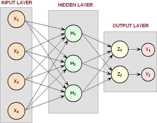
A multilayer feed-forward neural network is an interconnection of perceptrons in which data and calculations flow in a single direction, from the input data to the outputs. The number of layers in a neural network is the number of layers of perceptrons. The simplest neural network is one with a single input layer and an output layer of perceptrons. The network in Figure 7 illustrates this type of network. Technically this is referred to as a one-layer feed-forward network with two outputs because the output layer is the only layer with an activation calculation.
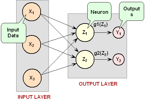
In this single-layer feed-forward neural network, the inputs are directly connected to the output layer perceptrons, \(Z_1\) and \(Z_2\).
The output perceptrons use activation functions, \(g_1\) and \(g_2\), to produce the outputs \(Y_1\) and \(Y_2\)
Since $$Z_1=\sum\limits_{i = 1}^3 {W_{1,i} } X_i -\mu _1$$ and $$Z_2=\sum\limits_{i = 1}^3 {W_{2,i}} X_i -\mu _2$$ $$Y_1=g_1(Z_1)=g_1(\sum\limits_{i=1}^3{W_{1,i}}X_i-\mu_1)$$ and $$Y_2=g_2 (Z_2 )=g_2(\sum\limits_{i=1}^3{W_{2,i}}X_i-\mu_2)$$ When the activation functions \(g_1\) and \(g_2\) are identity activation functions, a single-layer neural net is equivalent to a linear regression model. Similarly, if \(g_1\) and \(g_2\) are logistic activation functions, then the single-layer neural net is equivalent to logistic regression. Because of this correspondence between single-layer neural networks and linear and logistic regression, single-layer neural networks are rarely used in place of linear and logistic regression.
The next most complicated neural network is one with two layers. This extra layer is referred to as a hidden layer. In general there is no restriction on the number of hidden layers. However, it has been shown mathematically that a two-layer neural network, such as shown in Figure 1, can accurately reproduce any differentiable function, provided the number of perceptrons in the hidden layer is unlimited.
However, increasing the number of neurons increases the number of weights that must be estimated in the network, which in turn increases the execution time for this network. Instead of increasing the number of perceptrons in the hidden layer to improve accuracy, it is sometimes better to add additional hidden layers, which typically reduces both the total number of network weights and the computational time. However, in practice, it is uncommon to see neural networks with more than two or three hidden layers.
Neural Network Error Calculations
Error Calculations for Forecasting
The error calculations used to train a neural network are very important. Many error calculations have been researched, trying to find a calculation with a short training time that is appropriate for the network's application. Typically error calculations are very different depending primarily on the network's application.
For forecasting, the most popular error function is the sum-of-squared errors, or one of its scaled versions. This is analogous to using the minimum least squares optimization criterion in linear regression. Like least squares, the sum-of-squared errors is calculated by looking at the squared difference between what the network predicts for each training pattern and the target value, or observed value, for that pattern. Formally, the equation is the same as one-half the traditional least squares error:
$$E={\textstyle{1 \over 2}}\sum\limits_{i = 1}^N {\sum\limits_{j=1}^C{\left({t_{ij}-\hat t{}_{ij}} \right)^2}}$$where N is the total number of training cases, C is equal to the number of network outputs, \(t_{ij}\) is the observed output for the i-th training case and the j-th network output, and \(\hat t_{ij}\) is the network's forecast for that case.
Common practice recommends fitting a different network for each forecast variable. That is, the recommended practice is to use C=1 when using a multilayer feed-forward neural network for forecasting. For classification problems with more than two classes, it is common to associate one output with each classification category, i.e., C=number of classes.
Notice that in ordinary least squares, the sum-of-squared errors is not multiplied by one-half. Although this has no impact on the final solution, it significantly reduces the number of computations required during training.
Also note that as the number of training patterns increases, the sum-of-squared errors increases. As a result, it is often useful to use the root-mean-square (RMS) error instead of the unscaled sum-of-squared errors:
$$E^{RMS} = \frac{{\sum\limits_{i = 1}^N {\sum\limits_{j = 1}^C {\left( {t_{ij} - \hat t{}_{ij}} \right)^2 } } }}{{\sum\limits_{i = 1}^N {\sum\limits_{j = 1}^C {\left( {t_{ij} - \bar t} \right)^2 } } }} $$where \(\bar t\) is the average output:
$$\bar t = \frac{{\sum\limits_{i = 1}^N {\sum\limits_{j = 1}^C {t_{ij} } } }}{{N \cdot C}}$$Unlike the unscaled sum-of-squared errors, \(E^{RMS}\) does not increase as N increases. The smaller the value of \(E^{RMS}\) the closer the network is predicting its targets during training. A value of \(E^{RMS}=0\) indicates that the network is able to predict every pattern exactly. A value of \(E^{RMS}=1\) indicates that the network is predicting the training cases only as well as using the mean of the training cases for forecasting.
Notice that the root-mean-squared error is related to the sum-of-squared error by a simple scale factor: $$E^{RMS}=\frac{2}{{\bar t}}\cdot E$$ Another popular error calculation for forecasting from a neural network is the Minkowski-R error. The sum-of-squared error, \(E\), and the root-mean-squared error, \(E^{RMS}\), are both theoretically motivated by assuming the noise in the target data is Gaussian. In many cases, this assumption is invalid. A generalization of the Gaussian distribution to other distributions gives the following error function, referred to as the Minkowski-R error:
$$E^R=\sum\limits_{i=1}^N{\sum\limits_{j=1}^C{\left|{t_{ij}-\hat t{}_{ij}}\right|^R}}$$Notice that \(E^R=2E\) when R=2.
A good motivation for using \(E^R\) instead of \(E\) is to reduce the impact of outliers in the training data. The usual error measures, \(E\) and \(E^{RMS}\), emphasize larger differences between the training data and network forecasts since they square those differences. If outliers are expected, then it is better to de-emphasize larger differences. This can be done by using the Minkowski-R error with R=1. When R=1, the Minkowski-R error simplifies to the sum of absolute differences:
$$L=E^1=\sum\limits_{i = 1}^N{\sum\limits_{j=1}^C{\left|{t_{ij}-\hat t{}_{ij}} \right|}}$$L is also referred to as the Laplacian error. Its name is derived from the fact that it can be theoretically justified by assuming the noise in the training data follows a Laplacian rather than Gaussian distribution.
Of course, similar to E, L generally increases when the number of training cases increases. Similar to \(E^{RMS}\), a scaled version of the Laplacian error can be calculated using the following formula:
$$L^{RMS} = \frac{{\sum\limits_{i = 1}^N {\sum\limits_{j = 1}^C {\left| {t_{ij} - \hat t{}_{ij}} \right|} } }}{{\sum\limits_{i = 1}^N {\sum\limits_{j = 1}^C {\left| {t_{ij} - \bar t} \right|} } }}$$Cross-Entropy Error for Binary Classification
As previously mentioned, multilayer feed-forward neural networks can be used for both forecasting and classification applications. Training a forecasting network involves finding the network weights that minimize either the Gaussian or Laplacian distributions, E or L respectively, or equivalently their scaled versions, \(E^{RMS}\) or \(L^{RMS}\). Although these error calculations can be adapted for use in classification by setting the target classification variable to zeros and ones, this is not recommended. Use of the sum-of-squared and Laplacian error calculations is based on the assumption that the target variable is continuous. In classification applications, the target variable is a discrete random variable with C possible values, where C=number of classes.
A multilayer feed-forward neural network for classifying patterns into one of only two categories is referred to as a binary classification network. It has a single output: the estimated probability that the input pattern belongs to one of the two categories. The probability that it belongs to the other category is equal to one minus this probability, i.e.,
$$P(C_2)=P(\text{not}~C_1)=1-P(C_1)$$Binary classification applications are very common. Any problem requiring yes/no classification is a binary classification application. For example, deciding to sell or buy a stock is a binary classification problem. Deciding to approve a loan application is also a binary classification problem. Deciding whether to approve a new drug or to provide one of two medical treatments are binary classification problems.
For binary classification problems, only a single output is used, C=1. This output represents the probability that the training case should be classified as yes. A common choice for the activation function of the output of a binary classification network is the logistic activation function, which always results in an output in the range 0 to 1, regardless of the perceptron's potential.
One choice for training a binary classification network is to use sum-of-squared errors with the class value of yes patterns coded as a 1 and the no classes coded as a 0, i.e.: $$t_{ij} = \left\{ \begin{array}{cl} 1 & \text{if training pattern } i= \text{yes} \\ 0 & \text{if the training pattern } i= \text{no} \\ \end{array} \right.$$ However, using either the sum-of-squared or Laplacian errors for training a network with these target values assumes that the noise in the training data is Gaussian. In binary classification, the zeros and ones are not Gaussian. They follow the Bernoulli distribution: $$P(t_i=t)=p^t(1-p)^{1-t}$$ where p is equal to the probability that a randomly selected case belongs to the yes class.
Modeling the binary classes as Bernoulli observations leads to the use of the cross-entropy error function described by Hopfield (1987) and Bishop (1995):
$$E^C=-\sum\limits_{i=1}^N{\left\{{t_i\ln(\hat t_i)+(1-t_i)\ln(1-\hat t_i)}\right\}}$$where N is the number of training patterns, \(t_i\) is the target value for the i-th case (either 1 or 0), and \(\hat t_i\) is the network's output for the i-th case. This is equal to the neural network's estimate of the probability that the i-th case should be classified as yes.
For situations in which the target variable is a probability in the range \(0\lt t_{ij}\lt 1\), the value of the cross-entropy at the network's optimum is equal to: $$E_{\min }^C = - \sum\limits_{i = 1}^N {\left\{ {t_i \ln (t_i ) + (1 - t_i )\ln (1 - t_i )} \right\}} $$ Subtracting this from \(E^C\) gives an error term bounded below by zero, i.e., \(E^{CE} \ge 0\) where: $$E^{CE} = E^C - E_{\min }^C = - \sum\limits_{i = 1}^N {\left\{ {t_i \ln \left[ {\frac{{\hat t_i }}{{t_i }}} \right] + (1 - t_i )\ln \left[ {\frac{{1 - \hat t_i }}{{1 - t_i }}} \right]} \right\}}$$ This adjusted cross-entropy is normally reported when training a binary classification network where \(0 \lt t_{ij} \lt 1\). Otherwise \(E^C\), the non-adjusted cross-entropy error, is used. Small values, values near zero, would indicate that the training resulted in a network with a low error rate and that patterns are being classified correctly most of the time.
Cross-Entropy Error for Multi-Classification
Using a multilayer feedforward neural network for binary classification is relatively straightforward. A network for binary classification only has a single output that estimates the probability that an input pattern belongs to the yes class, i.e., \(t_i = 1\). In classification problems with more than two mutually exclusive classes, the calculations and network configurations are not as simple.
One approach is to use multiple network outputs, one for each of the C classes. Using this approach, the j-th output for the i-th training pattern, \(t_{ij}\), is the estimated probability that the i-th pattern is the network's j-th class, denoted by \(\hat{t}_{ij}\). An easy way to estimate these probabilities is to use logistic activation for each output. This ensures that each output satisfies the univariate probability requirements, i.e., \(0 \le \hat{t}_{ij} \le 1\).
However, since the classification categories are mutually exclusive, each pattern can only be assigned to one of the C classes, which means that the sum of these individual probabilities should always equal 1. However, if each output is the estimated probability for that class, it is very unlikely that \(\sum\limits_{j = 1}^C {\hat t_{ij} = 1}\). In fact, the sum of the individual probability estimates can easily exceed 1 if logistic activation is applied to every output.
Support Vector Machine (SVM) neural networks use this approach with one modification. An SVM network classifies a pattern as belonging to the i-th category if the activation calculation for that category exceeds a threshold and the other calculations do not exceed this value. That is, the i-th pattern is assigned to the j-th category if and if \(\hat t_{ij} > \delta \) and \(\hat t_{ik} \le \delta \) for all \(k \ne j\), where \(\delta\) is the threshold. If this does not occur, then the pattern is marked as unclassified.
Another approach to multi-class classification problems is to use the softmax activation function developed by Bridle (1990) on the network outputs. This approach produces outputs that conform to the requirements of a multinomial distribution. That is $$\sum\limits_{j = 1}^C {\hat t_{ij} = 1}$$ for all \(i = 1,2, \cdots ,N\) and \(0 \le \hat t_{ij} \le 1\) for all \(i = 1,2, \cdots ,N\) and \(j = 1,2, \cdots ,C\). The softmax activation function estimates classification probabilities using the following softmax activation function: $$\hat t_{ij} = \frac{{e^{Z_{ij} } }}{{\sum\limits_{j = 1}^C {e^{Z_{ij} } } }} $$ where \(Z_{ij}\) is the potential for the j-th output perceptron, or category, using the i-th pattern.
For this activation function, it is clear that:
- \(0 \le \hat t_{ij} \le 1\) for all \(i = 1,2, \cdots ,N\) and
- \(\sum\limits_{j = 1}^C {\hat t_{ij} = 1}\) for all \(i = 1,2, \cdots ,N\)
Modeling the C network outputs as multinomial observations leads to the cross-entropy error function described by Hopfield (1987) and Bishop (1995): $$E^C = - \sum\limits_{i = 1}^N {\sum\limits_{j = 1}^C {t_{ij} \ln (\hat t_{ij} )} } $$ where N is the number of training patterns, \(t_{ij}\) is the target value for the j-th class of i-th pattern (either 1 or 0), and \(\hat t_{ij}\) is the neural network's estimate of the j-th output for the i-th pattern. \(\hat t_{ij}\) is equal to the neural network's estimate of the probability that the i-th pattern should be classified into the j-th category.
For situations in which the target variable is a probability in the range \(0 \lt t_{ij} \lt 1\), the value of the cross-entropy at the networks optimum is equal to: $$ E_{\min }^C = - \sum\limits_{i = 1}^N {\sum\limits_{j = 1}^C {t_{ij} \ln (t_{ij} )} } $$ Subtracting this from \(E^C\) gives an error term bounded below by zero, i.e., \(E^{CE} \ge 0\) where: $$E^{CE} = E^C - E_{\min }^C = - \sum\limits_{i = 1}^N {\sum\limits_{j = 1}^C {t_{ij} \ln \left[ {\frac{{\hat t_{ij} }}{{t_{ij} }}} \right]} } $$ This adjusted cross-entropy is normally reported when training a binary classification network where \(0 \lt t_{ij} \lt 1\). Otherwise \(E^C\), the non-adjusted cross-entropy error, is used. That is, when 1-in-C encoding of the target variable is used, $$ t_{ij} = \left\{ {\begin{array}{*{20}c} 1 \hfill & {{\text{if the }}i{\text{-th pattern belongs to the }}j{\text{-th category}}} \hfill \\ 0 \hfill & {{\text{if the }}i{\text{-th pattern does not belong to the }}j{\text{-th category}}} \hfill \\ \end{array}} \right.$$ Small values, values near zero, indicate that the training resulted in a network with a low error rate and that patterns are being classified correctly most of the time.
Back-Propagation in Multilayer Feed-Forward Neural Network
Sometimes a multilayer feed-forward neural network is referred to incorrectly as a back-propagation network. The term back-propagation does not refer to the structure or architecture of a network. Back-propagation refers to the method used during network training. More specifically, back-propagation refers to a simple method for calculating the gradient of the network, that is the first derivative of the weights in the network.
The primary objective of network training is to estimate an appropriate set of network weights based upon a training dataset. There are many ways that have been researched for estimating these weights, but they all involve minimizing some error function. In forecasting, the most commonly used error function is the sum of squared errors:
$$E={\textstyle{1 \over 2}}\sum\limits_{i = 1}^N{\sum\limits_{j = 1}^C{\left( {t_{ij}- \hat t{}_{ij}}\right)^2 }}$$
Training uses one of several possible optimization methods to minimize this error term. Some of the more common are: steepest descent, quasi-Newton, conjugate gradient, and many various modifications of these optimization routines.
Back-propagation is a method for calculating the first derivative, or gradient, of the error function required by some optimization methods. It is certainly not the only method for estimating the gradient. However, it is the most efficient. In fact, some will argue that the development of this method by Werbos (1974), Parket (1985), and Rumelhart, Hinton and Williams (1986) contributed to the popularity of neural network methods by significantly reducing the network training time and making it possible to train networks consisting of a large number of inputs and perceptrons.
Simply stated, back-propagation is a method for calculating the first derivative of the error function with respect to each network weight. Bishop (1995) derives and describes these calculations for the two most common forecasting error functions, the sum of squared errors and Laplacian error functions. Abe (2001) gives the description for the classification error function, the cross-entropy error function. For all of these error functions, the basic formula for the first derivative of the network weight \(w_{ji}\) at the i-th perceptron applied to the output from the j-th perceptron $$\frac{{\partial E}}{{\partial w_{ji} }}=\delta _j Z_i, $$ where \(Z_i=g(a{}_i)\) is the output from the i-th perceptron after activation, and $$\frac{{\partial E}}{{\partial w_{ji}}}$$ is the derivative for a single output and a single training pattern. The overall estimate of the first derivative of \(w_{ji}\) is obtained by summing this calculation over all N training patterns and C network outputs.
The term back-propagation gets its name from the way the term \(\delta _j\) in the back-propagation formula is calculated: $$\delta _j=g'(a_j ) \cdot \sum\limits_k{w_{kj} \delta _k},$$ where the summation is over all perceptrons that use the activation from the j-th perceptron, \(g(a_j)\).
The derivative of the activation functions, \(g'(a)\), varies among these functions, see the following table:
| Activation Function | \(g(a)\) | \(g'(a)\) |
| Linear | \(g(a)=a\) | \(g'(a)=1\) (where a is a constant) |
| Logistic | \(g(a)=\frac{1}{{1+e^{-a}}}\) | \(g'(a)=g(a)(1-g(a))\) |
| Hyperbolic-tangent | \(g(a)=\text{tanh}(a)\) | \(g'(a)=\text{sech}^2 (a)=1-\text{tanh}^2(a)\) |
| Squash | \(g(a)=\frac{a}{{1+\left| a\right|}}\) | \(g'(a)=\frac{1}{{\left({1+\left| a\right|}\right)^2}}\) |