-
Interface Summary Interface Description DecisionTreeSurrogateMethod Methods to account for missing values in predictor variables. -
Class Summary Class Description ALACART Generates a decision tree using the CARTTM method of Breiman, Friedman, Olshen and Stone (1984).C45 Generates a decision tree using the C4.5 algorithm for a categorical response variable and categorical or quantitative predictor variables.CHAID Generates a decision tree using CHAID for categorical or discrete ordered predictor variables.DecisionTree Abstract class for generating a decision tree for a single response variable and one or more predictor variables.DecisionTreeInfoGain Abstract class that extendsDecisionTreefor classes that use an information gain criteria.QUEST Generates a decision tree using the QUEST algorithm for a categorical response variable and categorical or quantitative predictor variables.RandomTrees Generates predictions using a random forest of decision trees.Tree Serves as the root node of a decision tree and contains information about the relationship of child nodes.TreeNode ADecisionTreenode that is a child node ofTree. -
Enum Summary Enum Description DecisionTreeInfoGain.GainCriteria Specifies which information gain criteria to use in determining the best split at each node. -
Exception Summary Exception Description DecisionTree.MaxTreeSizeExceededException Exception thrown when the maximum tree size has been exceeded.DecisionTree.PruningFailedToConvergeException Exception thrown when pruning fails to converge.DecisionTree.PureNodeException Exception thrown when attempting to split a node that is already pure (response variable is constant).RandomTrees.ReflectiveOperationException Class that wraps exceptions thrown by reflective operations in core reflection.
Package com.imsl.datamining.decisionTree Description
Decision Trees - An Overview
Decision trees are data mining methods for predicting a single response variable based on multiple predictor variables. If the response variable is categorical or discrete, the data mining problem is a classification problem, whereas if the response is continuous, the problem is a type of regression problem. Decision trees are generally applicable in both situations.
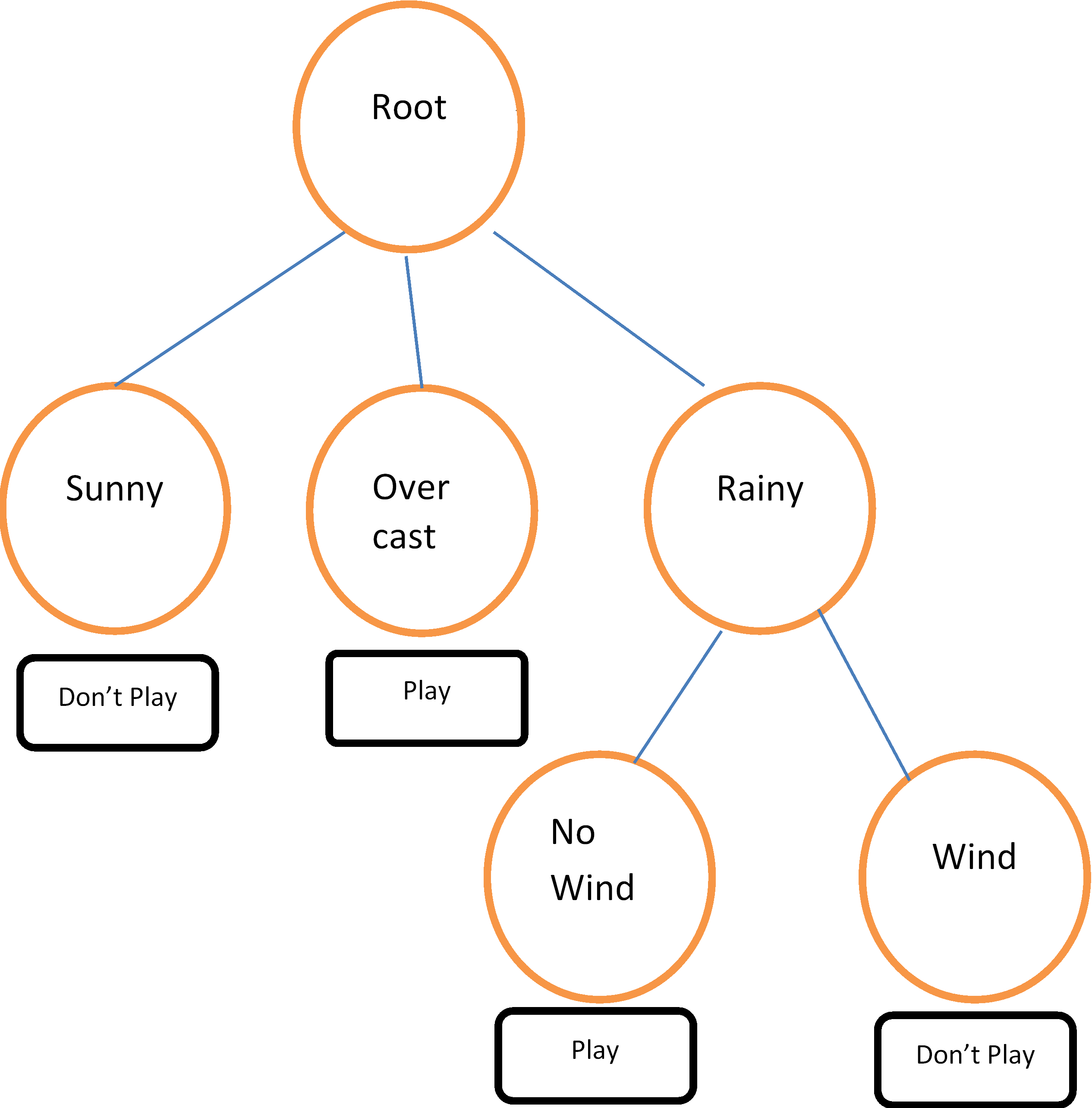
A simple example involves the decision to play golf or not, depending on the weather. The training data, from Quinlan (1993), is given in Table 30.1 and a decision tree fit to the data is shown in Figure 30.1. Other examples include predicting the chance of survival for heart attack patients based on age, blood pressure and other vital signs; scoring loan applications based on credit history, income, and education; classifying an email as spam based on its characteristics, and so on.
Tree-growing algorithms have similar steps: starting with all observations in a root node, a predictor variable is selected to split the dataset into two or more child nodes or branches. The form of the split depends on the type of predictor and on specifics of the algorithm. If the predictor is categorical, taking discrete values {A, B, C, D} for example, the split may consist of two or more proper subsets, such as {A}, {B, C}, and {D}. If the predictor is continuous, a split will consist of two or more intervals, such as \(X \le 2\), \(X \gt 2\). The splitting procedure is then repeated for each child node and continued in such manner until one of several possible stopping conditions is met. The result of the decision tree algorithm is a tree structure with a root and a certain number of branches (or nodes). Each branch defines a subset or partition of the data and, conditional on that subset of data, a predicted value for the response variable. A traversal of a branch of the tree thus leads to a prediction, or decision about the response variable. To predict a new observation, out-of-sample, we find the terminal node to which the observation belongs by traversing the tree and finding the data subset (branch) that contains the observation.
For example, the decision tree in Figure 1 can be expressed as a set of rules: If the weather is sunny, don't play golf. If the weather is overcast, play golf. If the weather is rainy and there is no wind, play golf. On the other hand, if it is rainy and windy, don't play golf.
Decision trees are intuitive and can be very effective predictive tools. As with any predictive model, a decision tree should be tested on hold-out datasets or refined using K-fold cross-validation to prevent over-fitting.
| Outlook | Temperature | Humidity | Wind | Play |
|---|---|---|---|---|
| sunny | 85 | 85 | false | don't play |
| sunny | 80 | 90 | true | don't play |
| overcast | 83 | 78 | false | play |
| rainy | 70 | 96 | false | play |
| rainy | 68 | 80 | false | play |
| rainy | 65 | 70 | true | don't play |
| overcast | 64 | 65 | true | play |
| sunny | 72 | 95 | false | don't play |
| sunny | 69 | 70 | false | play |
| rainy | 75 | 80 | false | play |
| sunny | 75 | 70 | true | play |
| overcast | 72 | 90 | true | play |
| overcast | 81 | 75 | false | play |
| rainy | 71 | 80 | true | don't play |
| overcast | 81 | 75 | false | play |
| rainy | 71 | 80 | true | don't play |