-
Interface Summary Interface Description BoundedLeastSquares.Function Public interface for the user-supplied function to evaluate the function that defines the least-squares problem.BoundedLeastSquares.Jacobian Public interface for the user-supplied function to compute the Jacobian.ConjugateGradient.Function Public interface for the user supplied function toConjugateGradient.ConjugateGradient.Preconditioner Public interface for the user supplied function toConjugateGradientused for preconditioning.FeynmanKac.Boundaries Public interface for user supplied boundary coefficients and terminal condition the PDE must satisfy.FeynmanKac.ForcingTerm Public interface for non-zero forcing term in the Feynman-Kac equation.FeynmanKac.InitialData Public interface for adjustment of initial data or as an opportunity for output during the integration steps.FeynmanKac.PdeCoefficients Public interface for user supplied PDE coefficients in the Feynman-Kac PDE.GenMinRes.Function Public interface for the user supplied function toGenMinRes.GenMinRes.Norm Public interface for the user supplied function to theGenMinResobject used for the norm \( \Vert X \Vert \) when the Gram-Schmidt implementation is used.GenMinRes.Preconditioner Public interface for the user supplied function toGenMinResused for preconditioning.GenMinRes.VectorProducts Public interface for the user supplied function to theGenMinResobject used for the inner product when the Gram-Schmidt implementation is used.HyperRectangleQuadrature.Function Public interface function for the HyperRectangleQuadrature class.MinConGenLin.Function Public interface for the user-supplied function to evaluate the function to be minimized.MinConGenLin.Gradient Public interface for the user-supplied function to compute the gradient.MinConNLP.Function Public interface for the user supplied function to theMinConNLPobject.MinConNLP.Gradient Public interface for the user supplied function to compute the gradient forMinConNLPobject.MinConNonlin.Function Deprecated MinConNonlinhas been replaced byMinConNLP.MinConNonlin.Gradient Deprecated MinConNonlinhas been replaced byMinConNLP.MinUncon.Derivative Public interface for the user supplied function to theMinUnconobject.MinUncon.Function Public interface for the user supplied function to theMinUnconobject.MinUnconMultiVar.Function Public interface for the user supplied function to theMinUnconMultiVarobject.MinUnconMultiVar.Gradient Public interface for the user supplied gradient to theMinUnconMultiVarobject.MinUnconMultiVar.Hessian Public interface for the user supplied Hessian to theMinUnconMultiVarobject.NelderMead.Function Public interface for the user-supplied function to evaluate the objective function of the minimization problem.NonlinLeastSquares.Function Public interface for the user supplied function to theNonlinLeastSquaresobject.NonlinLeastSquares.Jacobian Public interface for the user supplied function to theNonlinLeastSquaresobject.NumericalDerivatives.Function Public interface function.NumericalDerivatives.Jacobian Public interface for the user-supplied function to compute the Jacobian.OdeAdamsGear.Function Public interface for user supplied function toOdeAdamsGearobject.OdeAdamsGear.Jacobian Public interface for the user supplied function to evaluate the Jacobian matrix.OdeRungeKutta.Function Public interface for user supplied function toOdeRungeKuttaobject.Quadrature.Function Public interface function for the Quadrature class.RadialBasis.Function Public interface for the user supplied function to theRadialBasisobject.ZeroFunction.Function Deprecated ZeroFunctionhas been replaced byZerosFunction.ZerosFunction.Function Public interface for the user supplied function toZerosFunction.ZeroSystem.Function Public interface for user supplied function toZeroSystemobject.ZeroSystem.Jacobian Public interface for user supplied function toZeroSystemobject. -
Class Summary Class Description Bessel Collection of Bessel functions.BoundedLeastSquares Solves a nonlinear least-squares problem subject to bounds on the variables using a modified Levenberg-Marquardt algorithm.BoundedVariableLeastSquares Solve a linear least-squares problem with bounds on the variables.BsInterpolate Extension of the BSpline class to interpolate data points.BsLeastSquares Extension of the BSpline class to compute a least squares spline approximation to data points.BSpline BSpline represents and evaluates univariate B-splines.Cholesky Cholesky factorization of a matrix of typedouble.Complex Set of mathematical functions for complex numbers.ComplexEigen Collection of complex Eigen System functions.ComplexFFT Complex FFT.ComplexLU LU factorization of a matrix of typeComplex.ComplexMatrix Complex matrix manipulation functions.ComplexSparseCholesky Sparse Cholesky factorization of a matrix of typeComplexSparseMatrix.ComplexSparseCholesky.NumericFactor Data structures and functions for the numeric Cholesky factor.ComplexSparseCholesky.SymbolicFactor Data structures and functions for the symbolic Cholesky factor.ComplexSparseMatrix Sparse matrix of typeComplex.ComplexSparseMatrix.SparseArray TheSparseArrayclass uses public fields to hold the data for a sparse matrix in the Java Sparse Array format.ComplexSuperLU Computes the LU factorization of a general sparse matrix of typeComplexSparseMatrixby a column method and solves a sparse linear system of equations \(Ax=b\).ComplexSVD Singular Value Decomposition (SVD) of a rectangular matrix of typeComplex.ConjugateGradient Solves a real symmetric definite linear system using the conjugate gradient method with optional preconditioning.CsAkima Extension of the Spline class to handle the Akima cubic spline.CsInterpolate Extension of the Spline class to interpolate data points.CsPeriodic Extension of the Spline class to interpolate data points with periodic boundary conditions.CsShape Extension of the Spline class to interpolate data points consistent with the concavity of the data.CsSmooth Extension of the Spline class to construct a smooth cubic spline from noisy data points.CsSmoothC2 Extension of the Spline class used to construct a spline for noisy data points using an alternate method.CsTCB Extension of the Spline class to handle a tension-continuity-bias (TCB) cubic spline, also known as a Kochanek-Bartels spline and is a generalization of the Catmull-Rom spline.DenseLP Solves a linear programming problem using an active set strategy.Eigen Collection of Eigen System functions.EpsilonAlgorithm The class is used to determine the limit of a sequence of approximations, by means of the Epsilon algorithm of P.FeynmanKac Solves the generalized Feynman-Kac PDE.FFT FFT functions.GenMinRes Linear system solver using the restarted Generalized Minimum Residual (GMRES) method.GenMinRes.Formatter Deprecated UseIMSLFormatterinstead.Hyperbolic Pure Java implementation of the hyperbolic functions and their inverses.HyperRectangleQuadrature HyperRectangleQuadrature integrates a function over a hypercube.IEEE Pure Java implementation of the IEEE 754 functions as specified in IEEE Standard for Binary Floating-Point Arithmetic, ANSI/IEEE Standard 754-1985 (IEEE, New York).JMath Pure Java implementation of the standard java.lang.Math class.LinearProgramming Deprecated LinearProgramminghas been replaced byDenseLP.LU LU factorization of a matrix of typedouble.Matrix Manipulation methods for real-valued rectangular matrices.MinConGenLin Minimizes a general objective function subject to linear equality/inequality constraints.MinConNLP General nonlinear programming solver.MinConNLP.Formatter Deprecated UseIMSLFormatterinstead.MinConNonlin Deprecated MinConNonlinhas been replaced byMinConNLP.MinUncon Unconstrained minimization.MinUnconMultiVar Unconstrained multivariate minimization.NelderMead Minimizes a function of n variables with or without box constraints using a direct search polytope algorithm.NonlinLeastSquares Nonlinear least squares.NonNegativeLeastSquares Solves a linear least squares problem with nonnegativity constraints.NumericalDerivatives Compute the Jacobian matrix for a function \(f(y)\) with m components in n independent variables.ODE ODE represents and solves an initial-value problem for ordinary differential equations.OdeAdamsGear Extension of the ODE class to solve a stiff initial-value problem for ordinary differential equations using the Adams-Gear methods.OdeRungeKutta Solves an initial-value problem for ordinary differential equations using the Runge-Kutta-Verner fifth-order and sixth-order method.Physical Return the value of various mathematical and physical constants.PrintMatrix Matrix printing utilities.PrintMatrixFormat This class can be used to customize the actions of PrintMatrix.QR QR Decomposition of a matrix.QuadraticProgramming Solves the convex quadratic programming problem subject to equality or inequality constraints.Quadrature Quadratureis a general-purpose integrator that uses a globally adaptive scheme in order to reduce the absolute error.RadialBasis RadialBasis computes a least-squares fit to scattered data in \( {\bf R}^d\), where d is the dimension.RadialBasis.Gaussian The Gaussian basis function, \(e^{-ax^2}\).RadialBasis.HardyMultiquadric The Hardy multiquadric basis function, \(\sqrt{r^2+\delta^2} \).Sfun Collection of special functions.SparseCholesky Sparse Cholesky factorization of a matrix of typeSparseMatrix.SparseCholesky.NumericFactor The numeric Cholesky factorization of a matrix.SparseCholesky.SymbolicFactor The symbolic Cholesky factorization of a matrix.SparseLP Solves a sparse linear programming problem by an infeasible primal-dual interior-point method.SparseMatrix Sparse matrix of typedouble.SparseMatrix.SparseArray TheSparseArrayclass uses public fields to hold the data for a sparse matrix in the Java Sparse Array format.Spline Spline represents and evaluates univariate piecewise polynomial splines.Spline2D Represents and evaluates tensor-product splines.Spline2DInterpolate Computes a two-dimensional, tensor-product spline interpolant from two-dimensional, tensor-product data.Spline2DLeastSquares Computes a two-dimensional, tensor-product spline approximant using least squares.SuperLU Computes the LU factorization of a general sparse matrix of typeSparseMatrixby a column method and solves the real sparse linear system of equations \(Ax=b\).SVD Singular Value Decomposition (SVD) of a rectangular matrix of typedouble.SymEigen Computes the eigenvalues and eigenvectors of a real symmetric matrix.ZeroFunction Deprecated ZeroFunctionhas been replaced byZerosFunction.ZeroPolynomial The ZeroPolynomial class computes the zeros of a polynomial with complex coefficients, Aberth's method.ZerosFunction Finds the real zeros of a real, continuous, univariate function, f(x).ZeroSystem Solves a system of n nonlinear equations f(x) = 0 using a modified Powell hybrid algorithm. -
Enum Summary Enum Description ComplexMatrix.MatrixType Indicates which matrix type is used.Matrix.MatrixType Indicates which matrix type is used. -
Exception Summary Exception Description BoundedLeastSquares.FalseConvergenceException False convergence - The iterates appear to be converging to a noncritical point.BoundedVariableLeastSquares.TooManyIterException Maximum number of iterations exceeded.Cholesky.NotSPDException The matrix is not symmetric, positive definite.ComplexEigen.DidNotConvergeException The iteration did not converge.ComplexSparseCholesky.NotSPDException The matrix is not Hermitian, positive definite.ComplexSVD.DidNotConvergeException The iteration did not convergeConjugateGradient.NoConvergenceException The conjugate gradient method did not converge within the allowed maximum number of iterations.ConjugateGradient.NotDefiniteAMatrixException The input matrix A is indefinite, that is the matrix is not positive or negative definite.ConjugateGradient.NotDefiniteJacobiPreconditionerException The Jacobi preconditioner is not strictly positive or negative definite.ConjugateGradient.NotDefinitePreconditionMatrixException The Precondition matrix is indefinite.ConjugateGradient.SingularPreconditionMatrixException The Precondition matrix is singular.CsShape.TooManyIterationsException Too many iterations.DenseLP.AllConstraintsNotSatisfiedException All constraints are not satisfied.DenseLP.BoundsInconsistentException The bounds given are inconsistent.DenseLP.CyclingOccurringException The algorithm appears to be cycling.DenseLP.MultipleSolutionsException The problem has multiple solutions giving essentially the same minimum.DenseLP.NoAcceptablePivotException No acceptable pivot could be found.DenseLP.NoConstraintsAvailableException The LP problem has no constraints.DenseLP.ProblemUnboundedException The problem is unbounded.DenseLP.ProblemVacuousException The problem is vacuous.DenseLP.SomeConstraintsDiscardedException Some constraints were discarded because they were too linearly dependent on other active constraints.DenseLP.WrongConstraintTypeException Deprecated No longer used, replaced with anIllegalArgumentException.Eigen.DidNotConvergeException The iteration did not convergeFeynmanKac.BoundaryInconsistentException The boundary conditions are inconsistent.FeynmanKac.ConstraintsInconsistentException The constraints are inconsistent.FeynmanKac.CorrectorConvergenceException Corrector failed to converge.FeynmanKac.ErrorTestException Error test failure detected.FeynmanKac.InitialConstraintsException The constraints at the initial point are inconsistent.FeynmanKac.IterationMatrixSingularException Iteration matrix is singular.FeynmanKac.TcurrentTstopInconsistentException The end value for the integration in time, tout, is not consistent with the current time value, t.FeynmanKac.TEqualsToutException The current integration point in time and the end point are equal.FeynmanKac.TimeIntervalTooSmallException Distance between starting time point and end point for the integration is too small.FeynmanKac.ToleranceTooSmallException Tolerance is too small.FeynmanKac.TooManyIterationsException Too many iterations required by the DAE solver.GenMinRes.TooManyIterationsException Maximum number of iterations exceeded.LinearProgramming.BoundsInconsistentException Deprecated LinearProgramming.NumericDifficultyException Deprecated LinearProgramming.ProblemInfeasibleException Deprecated LinearProgramming.ProblemUnboundedException Deprecated LinearProgramming.WrongConstraintTypeException Deprecated No longer used, replaced with anIllegalArgumentException.MinConGenLin.ConstraintsInconsistentException The equality constraints are inconsistent.MinConGenLin.ConstraintsNotSatisfiedException No vector x satisfies all of the constraints.MinConGenLin.EqualityConstraintsException the variables are determined by the equality constraints.MinConGenLin.VarBoundsInconsistentException The equality constraints and the bounds on the variables are found to be inconsistent.MinConNLP.BadInitialGuessException Penalty function point infeasible for original problem.MinConNLP.ConstraintEvaluationException Constraint evaluation returns an error with current point.MinConNLP.IllConditionedException Problem is singular or ill-conditioned.MinConNLP.LimitingAccuracyException Limiting accuracy reached for a singular problem.MinConNLP.LinearlyDependentGradientsException Working set gradients are linearly dependent.MinConNLP.NoAcceptableStepsizeException No acceptable stepsize in [SIGMA,SIGLA].MinConNLP.ObjectiveEvaluationException Objective evaluation returns an error with current point.MinConNLP.PenaltyFunctionPointInfeasibleException Penalty function point infeasible.MinConNLP.QPInfeasibleException QP problem seemingly infeasible.MinConNLP.SingularException Problem is singular.MinConNLP.TerminationCriteriaNotSatisfiedException Termination criteria are not satisfied.MinConNLP.TooManyIterationsException Maximum number of iterations exceeded.MinConNLP.TooMuchTimeException Maximum time allowed for solve exceeded.MinConNLP.WorkingSetSingularException Working set is singular in dual extended QP.MinConNonlin.LineSearchException Deprecated MinConNonlinhas been replaced byMinConNLP.MinConNonlin.QPConstraintsException Deprecated MinConNonlinhas been replaced byMinConNLP.MinConNonlin.TooManyIterationsException Deprecated MinConNonlinhas been replaced byMinConNLP.MinConNonlin.UphillSearchCalcException Deprecated MinConNonlinhas been replaced byMinConNLP.MinConNonlin.ZeroSearchDirectionException Deprecated MinConNonlinhas been replaced byMinConNLP.MinUnconMultiVar.ApproximateMinimumException Scaled step tolerance satisfied; the current point may be an approximate local solution, or the algorithm is making very slow progress and is not near a solution, or the scaled step tolerance is too big.MinUnconMultiVar.FalseConvergenceException False convergence error; the iterates appear to be converging to a noncritical point.MinUnconMultiVar.MaxIterationsException Maximum number of iterations exceeded.MinUnconMultiVar.UnboundedBelowException Five consecutive steps of the maximum allowable stepsize have been taken, either the function is unbounded below, or has a finite asymptote in some direction or the maximum allowable step size is too small.NonlinLeastSquares.TooManyIterationsException Too many iterations.NonNegativeLeastSquares.TooManyIterException Maximum number of iterations has been exceeded.NonNegativeLeastSquares.TooMuchTimeException Maximum time allowed for solve is exceeded.OdeAdamsGear.DidNotConvergeException The iteration did not converge within the maximum number of steps allowed (default 500).OdeAdamsGear.MaxFcnEvalsExceededException Maximum function evaluations exceeded.OdeAdamsGear.SingularMatrixException The interpolation matrix is singular.OdeAdamsGear.ToleranceTooSmallException Tolerance is too small or the problem is stiff.OdeRungeKutta.DidNotConvergeException The iteration did not converge within the maximum number of steps allowed (default 500).OdeRungeKutta.ToleranceTooSmallException Tolerance is too small or the problem is stiff.QuadraticProgramming.InconsistentSystemException The system of constraints is inconsistent.QuadraticProgramming.NoLPSolutionException No solution for the LP problem with h = 0 was found byDenseLP.QuadraticProgramming.ProblemUnboundedException The objective value for the problem is unbounded.QuadraticProgramming.SolutionNotFoundException A solution was not found.SingularMatrixException The matrix is singular.SparseCholesky.NotSPDException The matrix is not symmetric, positive definite.SparseLP.CholeskyFactorizationAccuracyException The Cholesky factorization failed because of accuracy problems.SparseLP.DiagonalWeightMatrixException A diagonal element of the diagonal weight matrix is too small.SparseLP.DualInfeasibleException The dual problem is infeasible.SparseLP.IllegalBoundsException The lower bound is greater than the upper bound.SparseLP.IncorrectlyActiveException One or more LP variables are falsely characterized by the internal presolver.SparseLP.IncorrectlyEliminatedException One or more LP variables are falsely characterized by the internal presolver.SparseLP.InitialSolutionInfeasibleException The initial solution for the one-row linear program is infeasible.SparseLP.PrimalInfeasibleException The primal problem is infeasible.SparseLP.PrimalUnboundedException The primal problem is unbounded.SparseLP.ProblemUnboundedException The problem is unbounded.SparseLP.TooManyIterationsException The maximum number of iterations has been exceeded.SparseLP.ZeroColumnException A column of the constraint matrix has no entries.SparseLP.ZeroRowException A row of the constraint matrix has no entries.SVD.DidNotConvergeException The iteration did not convergeZeroPolynomial.DidNotConvergeException The iteration did not convergeZeroSystem.DidNotConvergeException The iteration did not converge.ZeroSystem.ToleranceTooSmallException Tolerance too smallZeroSystem.TooManyIterationsException Too many iterations.
Package com.imsl.math Description
Differential Equations
Ordinary Differential Equations
An ordinary differential equation is an equation involving one or more dependent variables called \(y_i\), one independent variable, t, and derivatives of the \(y_i\) with respect to t.
In the initial-value problem (IVP), the initial or starting values of the dependent variables \(y_i\) at a known value \(t = t_0\) are given. Values of \(y_i(t)\) for \(t \gt t_0\) or \(t \lt t_0\) are required.
The classes OdeRungeKutta and OdeAdamsGear solve the IVP for ODEs of the form
$$\frac{{dy_i }}{{dt}} = y'_i = f_i \left( {t,\,y_1 ,\,...\,,y_N } \right)\,\,\,\,\,\,\,\,\,\,i = 1,\,...\,,\,N$$
with \(y_i(t_0)\) specified. Here, \(f_i\) is a user-supplied function that must be evaluated at any set of values \((t, y_1, \ldots, y_N), i = 1, \ldots, N\).
This problem statement is abbreviated by writing it as a system of first-order ODEs,
$$y\left( t \right) = \left[ {y_1 \left( t \right), \ldots ,y_N \left ( t \right)} \right]^T , f(t,y) = \left[ {f_1 \left( {t,y} \right), \ldots ,f_N \left( {t,y} \right)} \right]^T$$
so that the problem becomes \(y' = f\left( {t,y} \right) \) with initial values \(y(t_0)\).
The system
$$\frac{{dy}}{{dt}} = y' = f\left( {t,y} \right)$$
is said to be stiff if some of the eigenvalues of the Jacobian matrix
$$\left\{ {\partial y'_i /\partial y_j } \right\}$$
are large and negative. This is frequently the case for differential equations modeling the behavior of physical systems, such as chemical reactions proceeding to equilibrium where subspecies effectively complete their reactions in different epochs. An alternate model concerns discharging capacitors such that different parts of the system have widely varying decay rates (or time constants).
Users typically identify stiff systems by the fact that numerical differential equation
solvers such as OdeRungeKutta are inefficient, or else completely fail. Special
methods are often required. The most common inefficiency is that a large number of evaluations
of f(t, y) (and hence an excessive amount of computer time) are required to satisfy the
accuracy and stability requirements of the software. In such cases, use OdeAdamsGear.
For more discussion about stiff systems, see Gear (1971, Chapter 11) or Shampine and Gear (1979).
Partial Differential Equations
The FeynmanKac class solves the Feynman-Kac equation, a single partial differential
equation, on a finite interval \([x_{\min},x_{\max}]\), for given grid points on the time
interval \( [ \hat{T}, T ] \). This equation often arises
in applications from financial engineering and that is the primary focus of the documentation
examples. The equation, initial conditions and Feynman-Kac boundary values are given by
$$
f_t+\mu(x,t)+\frac{\sigma^2(x,t)}{2}f_{xx}-\kappa(x,t)f = \phi(f,x,t)
$$
$$
f(x,T)=p(x)
$$
$$
a(x,t)f+b(x,t)f_x+c(x,t)f_{xx}=d(x,t), \; x = x_{\min} \text{ or } x = x_{\max}
$$
where
$$ f_t=\frac{\partial{f}}{\partial{t}}, f_{tt}=\frac{\partial^2{f}}{(\partial{t})^2}, \text{etc.} $$
Eigensystem Analysis
An ordinary linear eigensystem problem is represented by the equation \(Ax = \lambda x\) where A denotes an n x n matrix. The value \(\lambda\) is an eigenvalue and \(x \neq 0\) is the corresponding eigenvector. The eigenvector is determined up to a scalar factor. In all functions, we have chosen this factor so that x has Euclidean length one, and the component of x of largest magnitude is positive. If x is a complex vector, this component of largest magnitude is scaled to be real and positive. The entry where this component occurs can be arbitrary for eigenvectors having non-unique maximum magnitude values.
Error Analysis and Accuracy
Except in special cases, functions will not return the exact eigenvalue-eigenvector pair for the ordinary eigenvalue problem \(Ax = \lambda x\). Typically, the computed pair
$$\tilde x,\;\tilde \lambda$$
are an exact eigenvector-eigenvalue pair for a "nearby" matrix A + E. Information about E is known only in terms of bounds of the form \(\left\| E \right\|_2 \le f\left( n \right)\left\| A \right\|_2 \varepsilon\). The value of f(n) depends on the algorithm, but is typically a small fractional power of n. The parameter \(\varepsilon\) is the machine precision. By a theorem due to Bauer and Fike (see Golub and Van Loan 1989, p. 342),
$$\min \left| {\tilde \lambda - \lambda } \right| \le \kappa \left( X \right)\left\| E \right\|_2 \,\,\,\, {\rm{for\,\, all}} \, \lambda \, {\rm{in}} \, \sigma \left( A \right) $$
where \(\sigma(A)\) is the set of all eigenvalues of A (called the spectrum of A), X is the matrix of eigenvectors, \(\left\| \cdot \right\|_2\) is Euclidean length, and \(\kappa (X)\) is the condition number of X defined as \(\kappa \left( X \right) = \left\| X \right\|_2 \left\| {X^{ - 1} } \right\|_2\). If A is a real symmetric or complex Hermitian matrix, then its eigenvector matrix X is respectively orthogonal or unitary. For these matrices, \(\kappa(X) = 1\).
The accuracy of the computed eigenvalues
$$\tilde \lambda _j$$
and eigenvectors
$$\tilde x_j$$
can be checked by computing their performance index \(\tau\). The performance index is defined to be
$$\tau = \mathop {\max }\limits_{1 \le j \le n} \,\,\frac{{\left\| {A\tilde x_j - \tilde \lambda _j \tilde x_j } \right\|_2 }}{{n\varepsilon \left\| A \right\|_2 \left\| {\tilde x_j } \right\|_2 }}$$
where \(\varepsilon\) is again the machine precision.
The performance index \( \tau\) is related to the error analysis because
$$\left\| {E\tilde x_j } \right\|_2 = \left\| {A\tilde x_j - \tilde \lambda _j \tilde x_j } \right\|_2$$
where E is the "nearby" matrix discussed above.
While the exact value of \(\tau\) is precision and data dependent, the performance of an eigensystem analysis function is defined as excellent if \(\tau \lt 1\), good if \(1 \leq \tau \leq 100\), and poor if \(\tau \gt 100\). This is an arbitrary definition, but large values of \(\tau\) can serve as a warning that there is a significant error in the calculation.
If the condition number \(\kappa(X)\) of the eigenvector matrix X is large, there can be large errors in the eigenvalues even if \(\tau\) is small. In particular, it is often difficult to recognize near multiple eigenvalues or unstable mathematical problems from numerical results. This facet of the eigenvalue problem is often difficult for users to understand. Suppose the accuracy of an individual eigenvalue is desired. This can be answered approximately by computing the condition number of an individual eigenvalue(see Golub and Van Loan 1989, pp. 344-345). For matrices A, such that the computed array of normalized eigenvectors X is invertible, the condition number of \(\lambda_i\) is
$$\kappa _j = \left\| {e_j^T X^{ - 1} } \right\|,$$
the Euclidean length of the j-th row of \(X^{-1}\). Users can choose to compute this matrix using the class LU in "Linear Systems." An approximate bound for the accuracy of a computed eigenvalue is then given by \(\kappa _j \varepsilon \left\| A \right\|\). To compute an approximate bound for the relative accuracy of an eigenvalue, divide this bound by \(\left| {\lambda _j } \right|\).
Interpolation and Approximation
This section contains classes to interpolate and approximate data with cubic splines. Interpolation means that the fitted curve passes through all of the specified data points. An approximation spline does not have to pass through any of the data points. An approximating curve can therefore be smoother than an interpolating curve.
Cubic splines are smooth \(C^1\) or \(C^2\) fourth-order piecewise-polynomial (pp) functions. For historical and other reasons, cubic splines are the most heavily used pp functions.
This section contains five cubic spline interpolation classes and two
approximation classes. These classes are derived from the base class Spline,
which provides basic services, such as spline evaluation and integration.
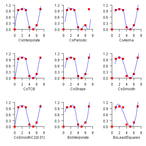
The chart shows how the nine splines in this section fit a single data set.
Class CsInterpolate allows
the user to specify various endpoint conditions (such as the value of the first
and second derivatives at the right and left endpoints).
Class CsPeriodic is used
to fit periodic (repeating) data. The sample data set used is not periodic and
so the curve does not pass through the final data point.
Class CsAkima keeps the
shape of the data while minimizing oscillations.
Class CsTCB allows
the user to specify various data point parameters (such as tension, continuity, and bias).
Class CsShape keeps the
shape of the data by preserving its convexity.
Class CsSmooth constructs a
smooth spline from noisy data.
Class CsSmoothC2 constructs
a smooth spline from noisy data using cross-validation and a user-supplied
smoothing parameter.
Class BSpline is the
abstract base class for univariate B-splines. B-splines provide a particularly
convenient and suitable basis for a given class of smooth piecewise polynomial
(ppoly) functions. Such a class is specified by giving its breakpoint sequence,
its order k, and the required smoothness across each of the interior
breakpoints. The corresponding B-spline basis is specified by giving its knot
sequence
\({\bf t} \in {\bf R}\). The specification rule is as follows:
if the class is to have all derivatives up to and including the j-th
derivative continuous across the interior breakpoint
\(\xi_i\), then the number
\(\xi_i\)
should occur k-j-1 times in the knot sequence. Assuming that
\(\xi_0\)
and
\(\xi_{n-1}\)
are the endpoints of the interval of interest, choose the first k knots
equal to
\(\xi_0\)
and the last k knots equal to
\(\xi_{n-1}\). This can be done because the B-splines are
defined to be right continuous near
\(\xi_0\)
and left continuous near
\(\xi_{n-1}\).
When the above construction is completed, a knot sequence t of length M is generated, and there are m = M-k B-splines of order k, for example \(B_0, \ldots, B_{m-1}\), spanning the ppoly functions on the interval with the indicated smoothness. That is, each ppoly function in this class has a unique representation \(p = a_0 B_0 + a_1 B_1 + \cdots + a_{m-1} B_{m-1}\) as a linear combination of B-splines. A B-spline is a particularly compact ppoly function. \(B_i\) is a nonnegative function that is nonzero only on the interval \([{\bf t}_i, {\bf t}_{i+k}]\) More precisely, the support of the i-th B-spline is \([{\bf t}_i, {\bf t}_{i+k}]\). No ppoly function in the same class (other than the zero function) has smaller support (i.e., vanishes on more intervals) than a B-spline. This makes B-splines particularly attractive basis functions since the influence of any particular B-spline coefficient extends only over a few intervals. When it is necessary to emphasize the dependence of the B-spline on its parameters, we will use the notation \(B_{i,k,t}\) to denote the i-th B-spline of order k for the knot sequence t.
Class BsInterpolate extends
BSpline
and creates a B-spline by interpolating data points.
Class BsLeastSquares extends
BSpline and creates a B-spline by computing a least squares spline
approximation to data points.
Class Spline2D is the
abstract base class for the two-dimensional, tensor-product splines.
Class Spline2DInterpolate
computes a Spline2D using interpolation from two-dimensional,
tensor-product data.
Class Spline2DLeastSquares
computes a Spline2D using least squares.
Class RadialBasis computes
an approximation to scattered data in
\({\bf R}^M\)
using radial-basis functions.
Nonlinear Equations
Zeros of a Polynomial
A polynomial function of degree n can be expressed as follows:
$$p(z) = a_nz^n + a_{n-1} z^{n-1} + \dots + a_1z + a_0$$
where \(a_n \neq 0\). The class ZeroPolynomial finds
zeros of a polynomial with real or complex coefficients using Aberth's method.
Zeros of a Function
The class ZerosFunction
uses Muller's method to find the real zeros of a real-valued function.
Root of System of Equations
A system of equations can be stated as follows:
$$ f_i(x) = 0, {\rm for}\,\,\,\,i = 1, 2, \ldots, n $$
where \(x \in {\bf R}^n\), and \(f_i : {\bf R^n \rightarrow R}
\). The ZeroSystem class uses a modified hybrid method due to M.J.D. Powell
to find the zero of a system of nonlinear equations.
Optimization
Unconstrained Minimization
The unconstrained minimization problem can be stated as follows:
$$\mathop {\min }\limits_{x\; \in \;R^n } f\left( x \right)$$
where \(f : {\bf R}^ {\it n} \rightarrow {\bf R}\) is continuous and has derivatives of all orders required by the algorithms. The functions for unconstrained minimization are grouped into three categories: univariate functions, multivariate functions, and nonlinear least-squares functions.
For the univariate functions, it is assumed that the function is unimodal within the specified interval. For discussion on unimodality, see Brent (1973).
The class MinUnconMultiVar finds the minimum of a multivariate
function using a quasi-Newton method. The default is to use a finite-difference
approximation of the gradient of f(x). Here, the gradient is defined to
be the vector
$$\nabla f\left( x \right) = \left[ {\frac{{\partial f\left( x \right)}} {{\partial x_1 }},\;\frac{{\partial f\left( x \right)}}{{\partial x_2 }},\;...\,,\;\frac{{\partial f\left( x \right)}}{{\partial x_n }}} \right]$$
However, when the exact gradient can be easily provided, the gradient should be
provided by implementing the interface MinUnconMultiVar.Gradient.
The NumericalDerivatives class can also be used in computing the
gradient for MinUnconMultiVar as well as other classes. For an
example, see NumericalDerivatives Example 6.
The nonlinear least-squares function uses a modified Levenberg-Marquardt algorithm. The most common application of the function is the nonlinear data-fitting problem where the user is trying to fit the data with a nonlinear model.
These functions are designed to find only a local minimum point. However, a function may have many local minima. Try different initial points and intervals to obtain a better local solution.
Linearly Constrained Minimization
The linearly constrained minimization problem can be stated as follows:
$$\begin{array}{c} \mathop {\min }\limits_{x\; \in \;R^n } f\left( x \right) \\ {\rm{subject \, to}} \\ A_1 x = b_1 \\ A_2 x \le b_2 \end{array}$$
where \(f : {\bf R}^{\it n} \rightarrow {\bf R}\), \(A_1\) and \(A_2\) are coefficient matrices, and \(b_1\) and \(b_2\) are vectors. If f(x) is linear, then the problem is a linear programming problem. If f(x) is quadratic, the problem is a quadratic programming problem.
The class SparseLP uses an infeasible primal-dual interior-point method
to solve sparse linear programming problems of all sizes. The constraint matrix is
stored in sparse coordinate storage format.
The class DenseLP uses an active set strategy to solve small- to
medium-sized linear programming problems. No sparsity is assumed since the
coefficients are stored in full matrix form.
The class QuadraticProgramming is designed to solve convex
quadratic programming problems using a dual quadratic programming algorithm. If
the given Hessian is not positive definite, then QuadraticProgramming
modifies it to be positive definite. In this case, output should be interpreted
with care because the problem has been changed slightly. Here, the Hessian of f(x)
is defined to be the n x n matrix
$$\nabla ^2 f\left( x \right) = \left[ {\frac{{\partial ^2 }} {{\partial x_i \partial x_j }}f\left( x \right)} \right] $$
The class MinConGenLin uses Powell's TOLMIN algorithm to solve
linear constrained problems for more general
objective functions (beyond linear and quadratic functions).
Nonlinearly Constrained Minimization
The nonlinearly constrained minimization problem can be stated as follows:
$$\begin{array}{l} \mathop {\min }\limits_{x\; \in \;R^n } f\left( x \right) \\ {\rm{subject \, to}} \,\,\, g_i \left( x \right) = 0 \,\,\,\, {\rm{for}} \,\,\, i = 1,\;2,\;\ldots\,,\;m_1 \\ g_i \left( x \right) \ge 0 \,\,\,\, {\rm{for}} \,\,\, i = m_1 + 1,\;\ldots\,,\;m \\ \end{array}$$
where \(f : {\bf R}^{\it n} \rightarrow \bf R\) and \(g_i : {\bf R}^{\it n} \rightarrow \bf R\), for \(i = 1, 2, \ldots, m\).
The class MinConNLP uses a sequential equality constrained
quadratic programming algorithm to solve this problem. A more complete
discussion of this algorithm can be found in the documentation.
Return Values from User-Supplied Functions
All values returned by user-supplied functions must be valid real numbers. It is the user's responsibility to check that the values returned by a user-supplied function do not contain NaN, infinity, or negative infinity values.
Example: Minimum of a smooth function
The minimum of \(e^x - 5x\) is found using function evaluations only.
import com.imsl.math.*;

public class OptimizationIntroEx1 {
    public static void main(String args[]) {
        MinUncon zf = new MinUncon();
        zf.setGuess(0.0);
        zf.setAccuracy(0.001);
        MinUncon.Function fcn = new MinUncon.Function() {
            public double f(double x) {
                double y = Math.exp(x) - 5.*x;
                if(!Double.isNaN(y)) {
                       return y;
                } else {
                       return 0.0;
                }
            }
        };
        System.out.println("Minimum is " + zf.computeMin(fcn));
    }
}
Transforms
Fast Fourier Transforms
A fast Fourier transform (FFT) is simply a discrete Fourier transform that is computed efficiently. Basically, the straightforward method for computing the Fourier transform takes approximately \(n^2\) operations where n is the number of points in the transform, while the FFT (which computes the same values) takes approximately \( n\log n \) operations. The algorithms in this section are modeled on the Cooley-Tukey (1965) algorithm. Hence, these functions are most efficient for integers that are highly composite; that is, integers that are a product of small primes.
For the two classes, FFT and ComplexFFT, a single instance can be used to transform multiple sequences of the same length. In this situation, the constructor computes the initial setup once. This may result in substantial computational savings. For more information on the use of these classes consult the documentation under the appropriate class name.
Continuous Versus Discrete Fourier Transform
There is, of course, a close connection between the discrete Fourier transform and the continuous Fourier transform. Recall that the continuous Fourier transform is defined (Brigham 1974) as
$$\hat f\left( \omega \right) = \left( {\Im f} \right)\left( \omega \right) = \int_{ - \infty }^\infty {f\left( t \right)} e^{ - 2\pi i\omega t} dt $$
We begin by making the following approximation:
$$\hat f\left( \omega \right) \approx \int_{ - T/2}^{T/2} {f\left( t \right)} e^{ - 2\pi i\omega t} dt$$
$$= \int_0^T {f\left( {t - T/2} \right)} e^{ - 2\pi i\omega \left( {t - T/2} \right)} dt$$
$$= e^{\pi i\omega T} \int_0^T {f\left( {t - T/2} \right)} e^{ - 2\pi i\omega t} dt$$
If we approximate the last integral using the rectangle rule with spacing \(h = T / n\) , we have
$$\hat f\left( \omega \right) \approx e^{\pi i\omega T} h\sum\limits_{k = 0}^{n - 1} {e^{ - 2\pi i\omega kh} } f\left( {kh - T/2} \right) $$
Finally, setting \(\omega = j/T\) for \(j = 0, \dots, n - 1\,\,\, \) yields
$$\hat f\left( {j/T} \right) \approx e^{\pi ij} h\sum\limits_{k = 0}^{n - 1} {e^{ - 2\pi ijk/n} } f\left( {kh - T/2} \right) = \left( { - 1} \right)^j \sum\limits_{k = 0}^{n - 1} {e^{ - 2\pi ijk/n} } f_k^h $$
where \(f_k^h\) denotes the \(k\)-th component of the vector
\(f^h = (f(-T/2), \dots, f( (n - 1)h - T/2))\)
.
Thus, after scaling the components by
\((-1)^h\)
, the discrete Fourier
transform, as computed in
ComplexFFT
(with input
\(f^h \)
) is
related to an approximation of the continuous Fourier transform by the above formula.