Usage Notes
The majority of the routines in this chapter produce piecewise polynomial or spline functions that either interpolate or approximate given data, or are support routines for the evaluation, integration, and conversion from one representation to another. Two major subdivisions of routines are provided. The cubic spline routines begin with the letters “CS” and utilize the piecewise polynomial representation described below. The B-spline routines begin with the letters “BS” and utilize the B-spline representation described below. Most of the spline routines are based on routines in the book by de Boor (1978).
Piecewise Polynomials
A univariate piecewise polynomial (function) p is specified by giving its breakpoint sequence
ξ ∈ Rn, the order k (degree k − 1) of its polynomial pieces, and the k × (n − 1) matrix c of its local polynomial coefficients. In terms of this information, the piecewise polynomial (pp) function is given by
ξ ∈ Rn, the order k (degree k − 1) of its polynomial pieces, and the k × (n − 1) matrix c of its local polynomial coefficients. In terms of this information, the piecewise polynomial (pp) function is given by
The breakpoint sequence ξ is assumed to be strictly increasing, and we extend the pp function to the entire real axis by extrapolation from the first and last intervals. The subroutines in this chapter will consistently make the following identifications for FORTRAN variables:
c = PPCOEF
ξ = BREAK
k = KORDER
N = NBREAK
This representation is redundant when the pp function is known to be smooth. For example, if p is known to be continuous, then we can compute c1,i+1 from the cji as follows
where Δξi := ξi+1 − ξi. For smooth pp, we prefer to use the irredundant representation in terms of the B-(for ‘basis’)-splines, at least when such a function is first to be determined. The above pp representation is employed for evaluation of the pp function at many points since it is more efficient.
Splines and B-splines
B-splines provide a particularly convenient and suitable basis for a given class of smooth pp functions. Such a class is specified by giving its breakpoint sequence, its order, and the required smoothness across each of the interior breakpoints. The corresponding B-spline basis is specified by giving its knot sequence t ∈ RM. The specification rule is the following: If the class is to have all derivatives up to and including the j-th derivative continuous across the interior breakpoint ξi, then the number ξi should occur k − j − 1 times in the knot sequence. Assuming that ξ1, and ξn are the endpoints of the interval of interest, one chooses the first k knots equal to ξ1 and the last k knots equal to ξn. This can be done since the B-splines are defined to be right continuous near ξ1 and left continuous near ξn.
When the above construction is completed, we will have generated a knot sequence t of length M; and there will be m := M − k B-splines of order k, say B1 ,…, Bm that span the pp functions on the interval with the indicated smoothness. That is, each pp function in this class has a unique representation
p = a1B1 + a2B2 + … + amBm
as a linear combination of B-splines. The B-spline routines will consistently make use of the following identifiers for FORTRAN variables:
a = BSCOEF
t = XKNOT
m = NCOEF
M = NKNOT
A B-spline is a particularly compact pp function. Bi is a nonnegative function that is nonzero only on the interval [ti, ti + k]. More precisely, the support of the i-th B-spline is [ti, ti + k]. No pp function in the same class (other than the zero function) has smaller support (i.e., vanishes on more intervals) than a B-spline. This makes B-splines particularly attractive basis functions since the influence of any particular B-spline coefficient extends only over a few intervals. When it is necessary to emphasize the dependence of the B-spline on its parameters, we will use the notation
Bi,k,t
to denote the i-th B-spline of order k for the knot sequence t.
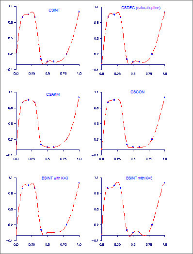
Figure 3, Spline Interpolants of the Same Data
Cubic Splines
Cubic splines are smooth (i.e., C 1 or C 2) fourth-order pp functions. For historical and other reasons, cubic splines are the most heavily used pp functions. Therefore, we provide special routines for their construction and evaluation. The routines for their determination use yet another representation (in terms of value and slope at all the breakpoints) but output the pp representation as described above for general pp functions.
We provide seven cubic spline interpolation routines: CSIEZ, CSINT, CSDEC, CSHER, CSAKM, CSCON, and CSPER. The first routine, CSIEZ, is an easy-to-use version of CSINT coupled with CSVAL. The routine CSIEZ will compute the value of the cubic spline interpolant (to given data using the ‘not-a-knot’ criterion) on a grid. The routine CSDEC allows the user to specify various endpoint conditions (such as the value of the first or second derivative at the right and left points). This means that the natural cubic spline can be obtained using this routine by setting the second derivative to zero at both endpoints. If function values and derivatives are available, then the Hermite cubic interpolant can be computed using CSHER. The two routines CSAKM and CSCON are designed so that the shape of the curve matches the shape of the data. In particular, CSCON preserves the convexity of the data while CSAKM attempts to minimize oscillations. If the data is periodic, then CSPER will produce a periodic interpolant. The routine CONFT allows the user wide latitude in enforcing shapes. This routine returns the B-spline representation.
It is possible that the cubic spline interpolation routines will produce unsatisfactory results. The adventurous user should consider using the B-spline interpolation routine BSINT that allows one to choose the knots and order of the spline interpolant.
In Figure 3, we display six spline interpolants to the same data. This data can be found in Example 1 of the IMSL routine CSCON Notice the different characteristics of the interpolants. The interpolation routines CSAKM and CSCON are the only two that attempt to preserve the shape of the data. The other routines tend to have extraneous inflection points, with the piecewise quartic (k = 5) exhibiting the most oscillation.
Tensor Product Splines
The simplest method of obtaining multivariate interpolation and approximation routines is to take univariate methods and form a multivariate method via tensor products. In the case of two-dimensional spline interpolation, the development proceeds as follows: Let tx be a knot sequence for splines of order kx, and ty be a knot sequence for splines of order ky. Let Nx + kx be the length of tx, and Ny + ky be the length of ty. Then, the tensor product spline has the form
Given two sets of points
for which the corresponding univariate interpolation problem could be solved, the tensor product interpolation problem becomes: Find the coefficients cnm so that
This problem can be solved efficiently by repeatedly solving univariate interpolation problems as described in de Boor (1978, page 347). Three-dimensional interpolation has analogous behavior. In this chapter, we provide routines that compute the two-dimensional tensor-product spline coefficients given two-dimensional interpolation data (BS2IN), compute the three-dimensional tensor-product spline coefficients given three-dimensional interpolation data (BS3IN) compute the two-dimensional tensor-product spline coefficients for a tensor-product least squares problem (BSLS2), and compute the three-dimensional tensor-product spline coefficients for a tensor-product least squares problem (BSLS3). In addition, we provide evaluation, differentiation, and integration routines for the two- and three-dimensional tensor-product spline functions. The relevant routines are BS2VL, BS3VL, BS2DR, BS3DR, BS2GD, BS3GD, BS2IG, and BS3IG.
Quadratic Interpolation
The routines that begin with the letters “QD” in this chapter are designed to interpolate a one-, two-, or three-dimensional (tensor product) table of values and return an approximation to the value of the underlying function or one of its derivatives at a given point. These routines are all based on quadratic polynomial interpolation.
Multi-dimensional Interpolation
We have one routine, SURF, that will return values of an interpolant to scattered data in the plane. This routine is based on work by Akima (1978), which utilizes C1 piecewise quintics on a triangular mesh. SURFND computes a piecewise polynomial interpolant, of up to 15-th degree, to a function of up to 7 variables, defined on a multi-dimensional grid.
Least Squares
Routines are provided to smooth noisy data: regression using linear regression using arbitrary polynomials (RCURV), and regression using user-supplied functions (FNLSQ). Additional routines compute the least-squares fit using splines with fixed knots (BSLSQ) or free knots (BSVLS). These routines can produce cubic-spline least-squares fit simply by setting the order to 4. The routine CONFT computes a fixed-knot spline weighted least-squares fit subject to linear constraints. This routine is very general and is recommended if issues of shape are important. The two- and three-dimensional tensor-product spline regression routines are (BSLS2) and (BSLS3).
Smoothing by Cubic Splines
Two “smoothing spline” routines are provided. The routine CSSMH returns the cubic spline that smooths the data, given a smoothing parameter chosen by the user. Whereas, CSSCV estimates the smoothing parameter by cross-validation and then returns the cubic spline that smooths the data. In this sense, CSSCV is the easier of the two routines to use. The routine CSSED returns a smoothed data vector approximating the values of the underlying function when the data are contaminated by a few random spikes.
Rational Chebyshev Approximation
The routine RATCH computes a rational Chebyshev approximation to a user-supplied function. Since polynomials are rational functions, this routine can be used to compute best polynomial approximations.
Using the Univariate Spline Routines
An easy to use spline interpolation routine CSIEZ is provided. This routine computes an interpolant and returns the values of the interpolant on a user-supplied grid. A slightly more advanced routine SPLEZ computes (at the users discretion) one of several interpolants or least-squares fits and returns function values or derivatives on a user-supplied grid.
For more advanced uses of the interpolation (or least squares) spline routines, one first forms an interpolant from interpolation (or least-squares) data. Then it must be evaluated, differentiated, or integrated once the interpolant has been formed. One way to perform these tasks, using cubic splines with the ‘not-a-knot’ end condition, is to call CSINT to obtain the local coefficients of the piecewise cubic interpolant and then call CSVAL to evaluate the interpolant. A more complicated situation arises if one wants to compute a quadratic spline interpolant and then evaluate it (efficiently) many times. Typically, the sequence of routines called might be BSNAK (get the knots), BSINT (returns the B-spline coefficients of the interpolant), BSCPP (convert to pp form), and PPVAL (evaluate). The last two calls could be replaced by a call to the B-spline grid evaluator BS1GD, or the last call could be replaced with pp grid evaluator PP1GD. The interconnection of the spline routines is summarized in Figure 4.
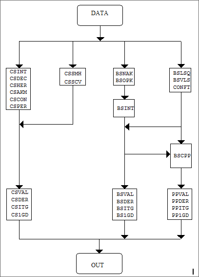
Figure 4, Interrelation of the Spline Routines
Choosing an Interpolation Routine
The choice of an interpolation routine depends both on the type of data and on the use of the interpolant. We provide 19 interpolation routines. These routines are depicted in a decision tree in Figure 3-3. This figure provides a guide for selecting an appropriate interpolation routine. For example, if periodic one-dimensional (univariate) data is available, then the path through univariate to periodic leads to the IMSL routine CSPER, which is the proper routine for this setting. The general-purpose univariate interpolation routines can be found in the box beginning with CSINT. Multidimensional tensor-product interpolation routines are also provided. For two-dimensional scattered data, the appropriate routine is SURF.
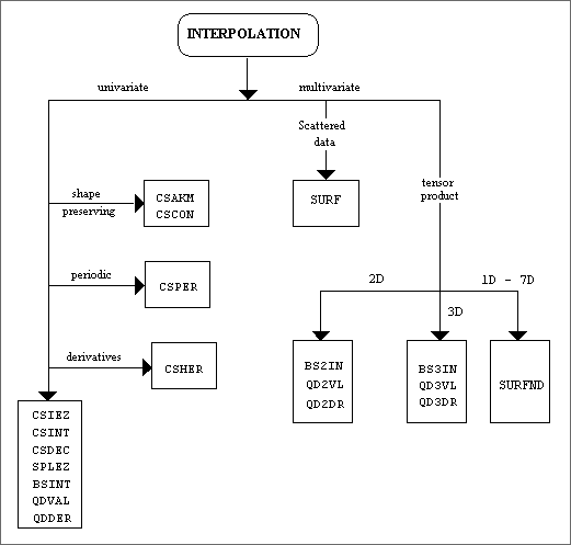
Figure 5, Choosing an Interpolation Routine
Published date: 03/19/2020
Last modified date: 03/19/2020


