Usage Notes
Comments
Definitions and discussions of the terms basic to this chapter can be found in Johnson and Kotz (1969, 1970a, 1970b). These are also good references for the specific distributions.
In order to keep the calling sequences simple, whenever possible, the subprograms described in this chapter are written for standard forms of statistical distributions. Hence, the number of parameters for any given distribution may be fewer than the number often associated with the distribution. For example, while a gamma distribution is often characterized by two parameters (or even a third, “location”), there is only one parameter that is necessary, the “shape”. The “scale” parameter can be used to scale the variable to the standard gamma distribution. Also, the functions relating to the normal distribution, ANORDF and ANORIN, are for a normal distribution with mean equal to zero and variance equal to one. For other means and variances, it is very easy for the user to standardize the variables by subtracting the mean and dividing by the square root of the variance.
The cumulative distribution function for the (real, single‑valued) random variable X is the function F defined for all real x by
F(x) = Prob(X ≤ x)
where Prob(⋅) denotes the probability of an event. The distribution function is often called the cumulative distribution function (CDF).
For distributions with finite ranges, such as the beta distribution, the CDF is 0 for values less than the left endpoint and 1 for values greater than the right endpoint. The subprograms described in this chapter return the correct values for the distribution functions when values outside of the range of the random variable are input, but warning error conditions are set in these cases.
Discrete Random Variables
For discrete distributions, the function giving the probability that the random variable takes on specific values is called the probability function, defined by
p(x) = Prob(X = x)
The “PR” routines described in this chapter evaluate probability functions.
The CDF for a discrete random variable is
where A is the set such that k ≤ x. The “DF” routines in this chapter evaluate cumulative distribution functions. Since the distribution function is a step function, its inverse does not exist uniquely.

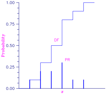
Figure 22, Discrete Random Variable
In the plot above, a routine like BINPR in this chapter evaluates the individual probability, given X. A routine like BINDFwould evaluate the sum of the probabilities up to and including the probability at X.
Continuous Distributions
For continuous distributions, a probability function, as defined above, would not be useful because the probability of any given point is 0. For such distributions, the useful analog is the probability density function (PDF). The integral of the PDF is the probability over the interval, if the continuous random variable X has PDF f, then
The relationship between the CDF and the PDF is
as shown in Figure 17‑2.

Figure 23, Probability Density Function
The “DF” routines described in this chapter evaluate cumulative distribution functions.
For (absolutely) continuous distributions, the value of F(x) uniquely determines x within the support of the distribution. The “IN” routines described in this chapter compute the inverses of the cumulative distribution functions, that is, given P =F(x) (called “P” for “probability”), a routine such as BETIN computes x. The inverses are defined only over the open interval (0,1).

Figure 24, Cumulative Probability Distribution Function
There are three routines described in this chapter that deal with general continuous distribution functions. The routine GCDF computes a distribution function using values of the density function, and the routine GCIN computes the inverse. These two routines may be useful when the user has an estimate of a probability density, as perhaps computed by the routine DESPL or DESKN (see Chapter 15: “Density and Hazard Estimation”), or computed from a frequency polygon. The routine GFNIN computes the inverse of a distribution function that is specified as a FORTRAN function.
Parameter Estimation
A related task to evaluating a probability density or distribution function is to estimate the values of its parameters. For many of the distributions covered in this chapter, routine MLE provides maximum likelihood estimates of the unknown parameter values given a sample of observations.
Additional Comments
Whenever a probability close to 1.0 results from a call to a distribution function or is to be input to an inverse function, it is often impossible to achieve good accuracy because of the nature of the representation of numeric values. In this case, it may be better to work with the complementary distribution function (one minus the distribution function). If the distribution is symmetric about some point (as the normal distribution, for example) or is reflective about some point (as the beta distribution, for example), the complementary distribution function has a simple relationship with the distribution function. For example, to evaluate the standard normal distribution at 4.0, using ANORIN directly, the result to six places is 0.999968. Only two of those digits are really useful, however. A more useful result may be 1.000000 minus this value, which can be obtained to six significant figures as 3.16713E‑05 by evaluating ANORIN at ‑4.0. For the normal distribution, the two values are related by Φ(x) = 1 ‑ Φ(‑x), where Φ(⋅) is the normal distribution function. Another example is the beta distribution with parameters 2 and 10. This distribution is skewed to the right, so evaluating BETDF at 0.7, we obtain 0.999953. A more precise result is obtained by evaluating BETDF with parameters 10 and 2 at 0.3. This yields 4.72392E‑5. (In both of these examples, it is wise not to trust the last digit.)
Many of the algorithms used by routines in this chapter are discussed by Abramowitz and Stegun (1964). The algorithms make use of various expansions and recursive relationships and often use different methods in different regions.
Cumulative distribution functions are defined for all real arguments, however, if the input to one of the distribution functions in this chapter is outside the range of the random variable, an error of Type 1 is issued, and the output is set to zero or one, as appropriate. A Type 1 error is of lowest severity, a “note”, and, by default, no printing or stopping of the program occurs. The other common errors that occur in the routines of this chapter are Type 2, “alert”, for a function value being set to zero due to underflow, Type 3, “warning”, for considerable loss of accuracy in the result returned, and Type 5, “terminal”, for incorrect and/or inconsistent input, complete loss of accuracy in the result returned, or inability to represent the result (because of overflow). When a Type 5 error occurs, the result is set to NaN (not a number, also used as a missing value code, obtained by routine AMACH(6). (See the section “User Errors” in the Reference Material.)
Published date: 03/19/2020
Last modified date: 03/19/2020


